Introduction
Last year, we used machine learning to predict the best shooters in the 2018 draft. Out of the players we analyzed, six of them ended up playing enough minutes that we could check how well the models predicted their PPG.
The six players who played enough for us to evaluate were Collin Sexton, Miles Bridges, Kevin Knox, Jaren Jackson Jr., Trae Young, and Mikal Bridges. For Sexton, Knox, and Jackson, the models were spot on; Sexton’s predicted PPG came in at 15.5, only 1.2 less than his actual PPG. Meanwhile, Knox and Jackson’s predictions came in at 0.7 and 2.2 PPG less than their actual scoring output. The models were not far from predicting Mikal Bridges’ PPG (11.3 predicted vs. 8.3 actual).
Trae Young and Miles Bridges had the biggest difference between predicted and actual PPG. Viewing Young as an inefficient volume scorer in college, the models predicted he would score only 11.5 PPG – 7.6 below his actual output of 19.1 PPG. On the opposite side, Miles Bridges turned in an efficient college career while averaging 17.0 PPG against good teams. This led the models to give him the second highest predicted PPG (behind only Sexton) at 13.0 – 5.5 above his actual output of 7.5 PPG.
Altogether, the predictions were not bad. The mean absolute error (average of the absolute value of the predicted – actual PPG) of the predictions was only 3.39, and the root mean squared error (root of the average of the predicted – actual PPG squared) was 4.17).
This year, we’ll improve our analysis significantly. We’ll use more advanced models and techniques. Additionally, we’ll predict PPG for all players projected to go in the first round (not just players who made at least 1 3-pointer per game in college).
Methods
The NCAA added a 3-point line for the 1986-1987 season, seven years after its introduction in the NBA. So, players drafted in 1990 played their entire college careers with a 3-point line. I created a database of the college stats for every player drafted in the first round since 1990. Sports-Reference provided all the college data, while Basketball-Reference provided all the NBA data.
In last year’s analysis, I made three big mistakes:
- I used every player’s NBA career PPG. Because at least 100 players in the data set have yet to reach their primes, using career PPG messes up the data. It combines people who lasted a full career with those who entered the league recently.
- I did not include the pick at which the player was taken. This is important because NBA GMs are good talent evaluators; generally, players picked earlier are better. There’s another hidden important factor with the pick: earlier picks often get more minutes and opportunities. If they’re given more opportunities, they will score more. This proved to be a big issue last year. Because pick was not included, several late first-round players had a high projected PPG. It’s unreasonable to predict a late-pick player to score 10 PPG given that he’s unlikely to even play 10 MPG.
- I limited the training data set to players who played at least half of their possible games and averaged at least 1 3PM. This removed many busts from the data set. Bad players won’t last to play that many games or make enough threes. This small data set also limited the models’ ability to learn.
To fix these issues, I made the models predict every player’s rookie year PPG, included draft pick as an input in the model, and used every first-round pick since 1990. In total, each model had seven inputs:
| Counting stats | Efficiency | Other |
|---|---|---|
| PPG | eFG% | Pick |
| FT% | SOS (strength of schedule) | |
| 3PAr | ||
| FTr |
With these inputs, I made 4 models:
- Support vector machine regression (SVM)
- Random forest regression (RF)
- k-nearest neighbors regression (KNN)
- Extreme gradient boosting regression (XGB)
These models will predict rookie year PPG for all first-round players in the Ringer’s 6/15 mock draft (link). Players who did not play in college are not included in this analysis given that we can’t compare NCAA and international stats. So, Sekou Doumbouya and Goga Bitadze are excluded.
Separating by position?
In a previous draft analysis where we predicted DBPM for all first-round players, we separated everything by position. We made separate models for guards, forwards, and centers given the very different defensive qualities required from each position. While steals from a center are nice, they’re not as important as blocks; the opposite is true for guards.
It may seem natural to split up by position here, too given that different positions score in different ways. Most notably, this difference is in 3-point shooting. However, in the modern basketball era, big men shoot 3-pointers at a high rate. Furthermore, 3-point percentage is not a model input. Instead, we use effective field goal percentage such that being inside scorers or rim-runner won’t hurt a player’s predicted PPG.
When I first ran the analysis, I tried splitting it up by guards, forwards, and centers. The models had very poor accuracy when split up by position. They performed much better when considering all players together. Therefore, we took all the players together in each of the models.
Regression analysis
Basic goodness-of-fit and cross-validation
As usual, we’ll begin our model discussion by examining the r-squared and mean squared error. Higher r-squared is better. The opposite is true for mean squared error.
The table below shows the r-squared and mean squared error for each of the four models.
| Model | r-squared | Mean squared error |
|---|---|---|
| SVM | 0.462 | 12.836 |
| RF | 0.499 | 11.959 |
| KNN | 0.508 | 11.742 |
| XGB | 0.511 | 11.679 |
Though the r-squared for each of the models is very poor, the mean squared error indicates the models can be accurate. The root mean squared error for each model is around 3.5. This is about 16% better than what last year’s models ended up having (4.17 root mean squared error). We saw that those models were spot on with their predictions for multiple players. Therefore, it’s likely these models will be as good as last year’s if not better.
Next, we’ll perform k-fold cross-validation to check that the models aren’t overfitting, or learning the data set “too well” to the point they won’t predict well on other data sets. We’d like the cross-validated r-squared to be close to (within the confidence interval) the actual r-squared seen above. This shows that the models perform similarly when used on a different split of the same data.
The table below shows the cross-validated r-squared scores and their 95% confidence intervals.
| Model | CV r-squared | Mean squared error |
|---|---|---|
| SVM | 0.42 | +/- 0.23 |
| RF | 0.41 | +/- 0.33 |
| KNN | 0.42 | +/- 0.20 |
| XGB | 0.37 | +/- 0.30 |
Each model has only a marginally higher true r-squared than cross-validated r-squared. So, the models shouldn’t perform much worse when we predict PPG for the 2019 draft class.
Standardized residuals test
The standardized residuals test adjusts the differences between predicted and actual values. When a model has at least 95% of its standardized residuals within 2 standard deviations of the mean, it passes the test. Passing the test tells us the model’s errors could be random (which is good).
The graph below shows the standardized residuals of all four models.

Every model passes the test. The only cause for concern is the large number of residuals with a magnitude greater than 2. The draft’s random nature likely contributes to this. Even so, the results of the standardized residuals test are encouraging.
Q-Q plot
Unlike the standardized residuals test, which examines if errors are random, a Q-Q (quantile-quantile) plot checks if the errors are normally distributed. This shows that the model’s errors are consistent across the entire data set.
A Q-Q plot for normally distributed residuals will have a 45-degree (y = x) line. The graph below is the Q-Q plot for all four models’ residuals.
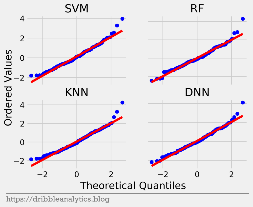
All four models have residuals close to the red y = x line for most of the quantiles. However, at the upper quantiles, there are noticeable jumps between the points. Furthermore, at the lowest quantiles, the residuals rise above the y = x line. Therefore, the residuals are probably not normally distributed.
Shapiro-Wilk test
To give a mathematical interpretation of what we’re trying to see with the Q-Q plot, we can use the Shapiro-Wilk test. The test returns a W-value between 0 and 1; 1 means the sample is perfectly normal.
Along with the W-Value, the Shapiro-Wilk test has a p-value, or probability that we can reject the null hypothesis. In this case, the null hypothesis is that the data is normally distributed. So, a p-value < 0.05 indicates that the residuals are not normally distributed (as p < 0.05 means we reject the null hypothesis).
The table below shows the results of the Shapiro-Wilk test.
| Model | W-value | p-value |
|---|---|---|
| SVM | 0.98 | < 0.01 |
| RF | 0.98 | < 0.01 |
| KNN | 0.97 | < 0.01 |
| XGB | 0.98 | 0.02 |
Though all four models have high W-values, they all have p-values < 0.05. This indicates that we can reject the null hypothesis of normality. Although this isn’t a positive result, it doesn’t make the models useless.
Results
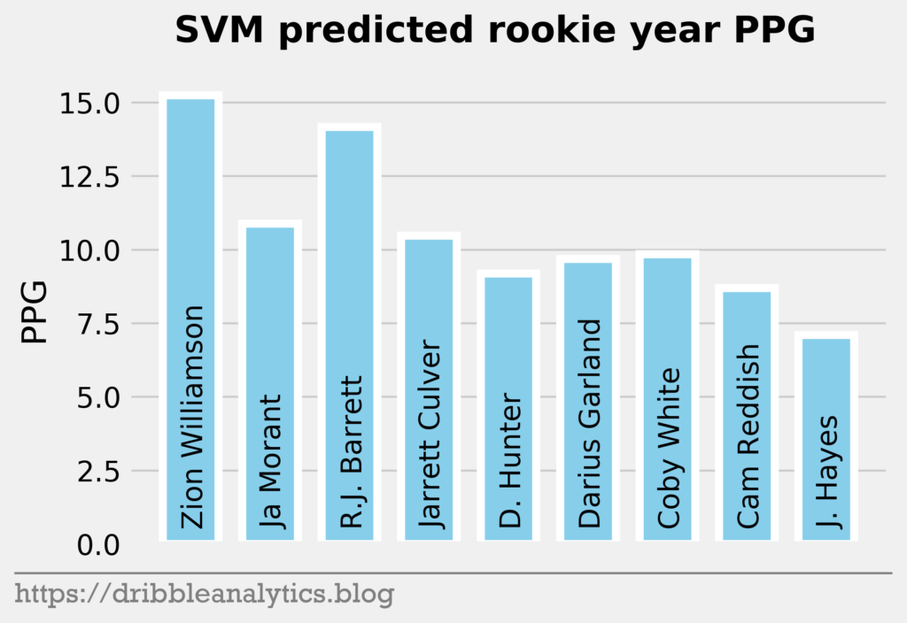
Aside from Sekou Doumbouya and Goga Bitadze, every first-round player in the Ringer’s mock draft played in college. So, we’ll predict PPG for 28/30 predicted first-round players. For each model, we’ll separate the predictions into three graphs: players projected 1-9, 10-18, and 19-28.
The bars are organized by projected pick (left-most player in range = earliest pick in the range).
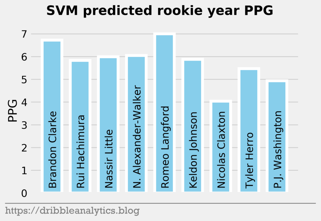
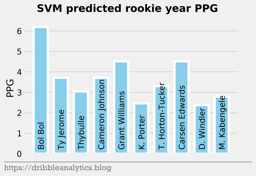
The three graphs below show the SVM predictions.
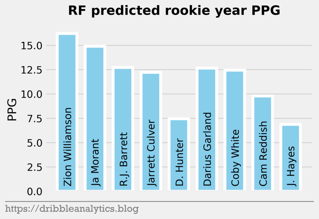
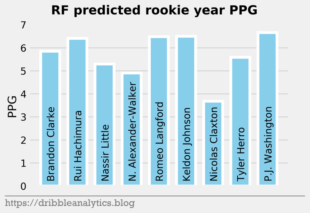
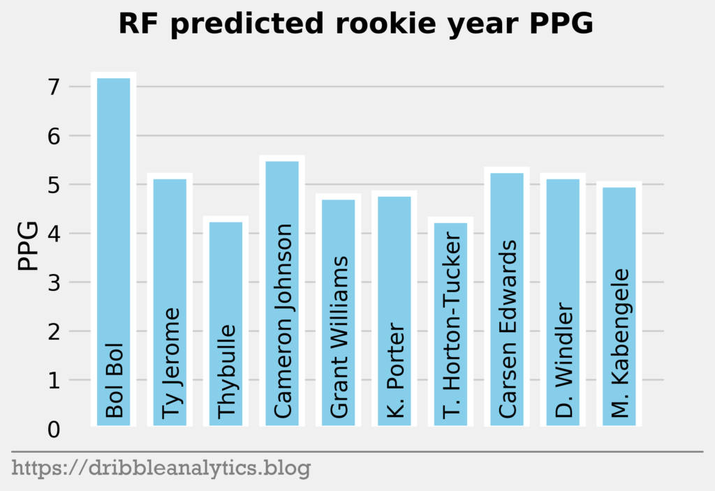
The three graphs below show the RF predictions.
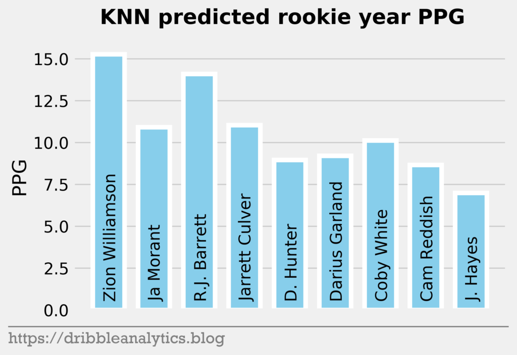
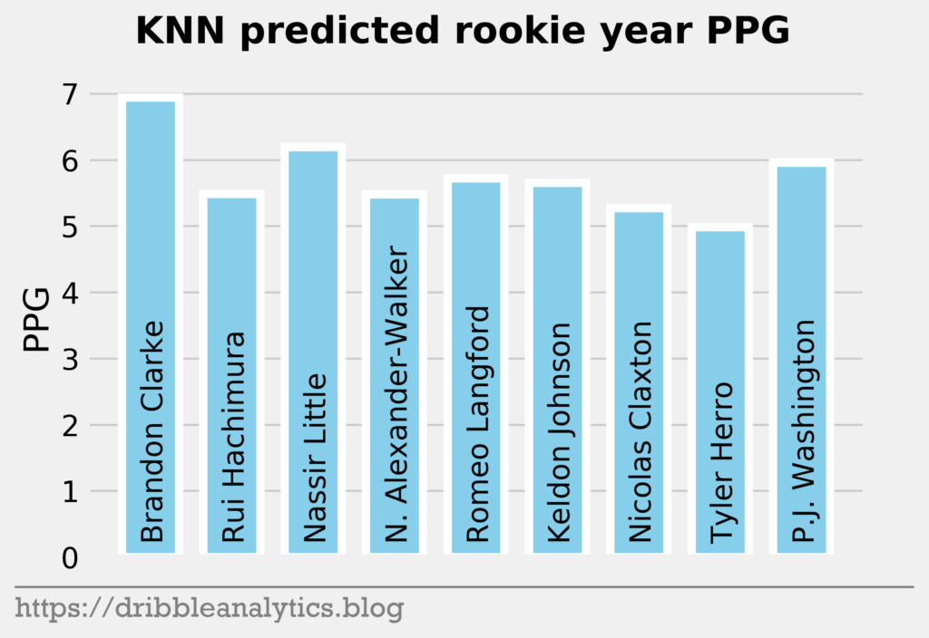
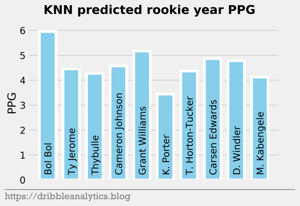
The three graphs below show the KNN predictions.
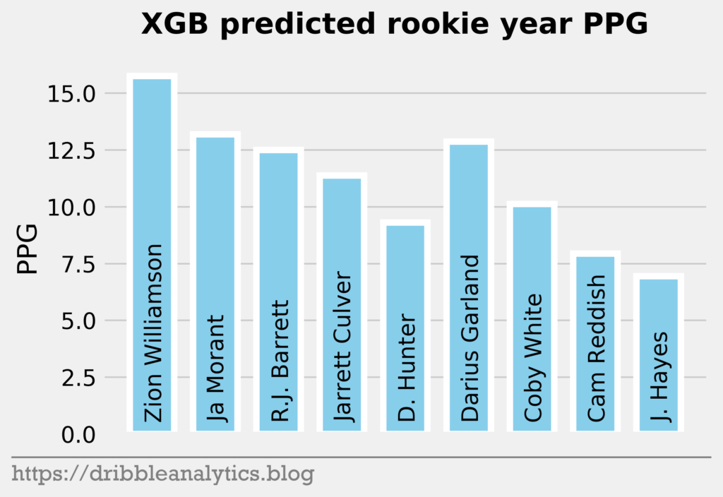
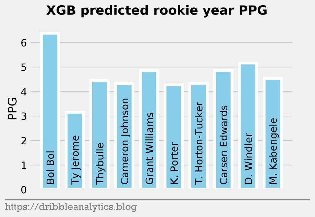
The three graphs below show the XGB predictions.

Average prediction
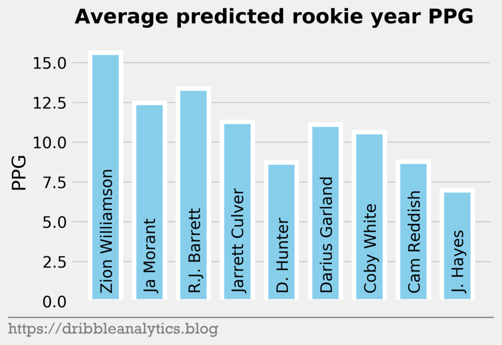
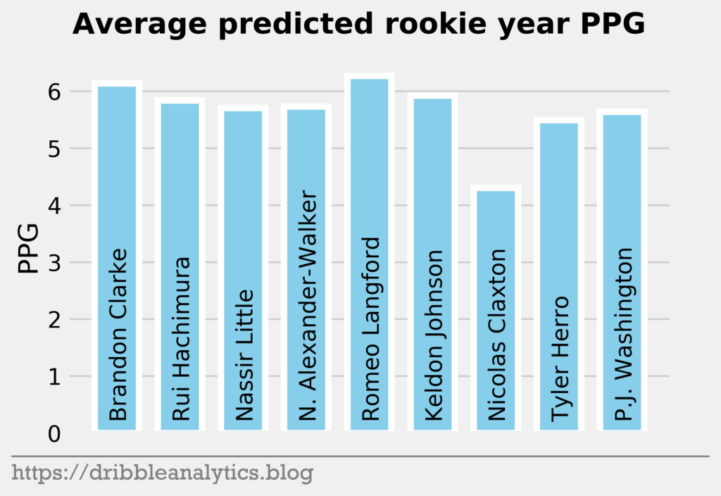
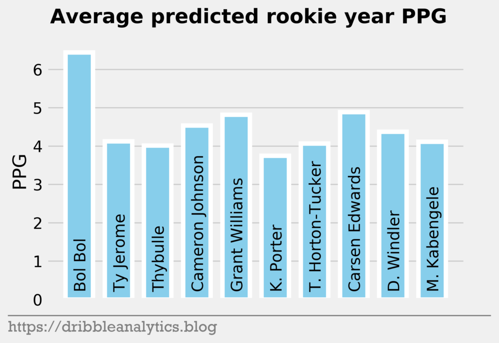
The three graphs below show the average prediction of the four models.
What impacts the models’ predictions?
All these models appear mysterious in their predictions. Though we know what factors go in and what comes out, we don’t know how each model weighs each factor for each prediction.
To see how much each input influences the models, we’ll use something called Shapley values. Shapley value is defined as the “average marginal contribution of a feature value over all possible coalitions.” So, it evaluates every prediction for an instance using every combo of the inputs. This method combined with other similar methods gives us more information about how much each individual feature affects each model in each case.
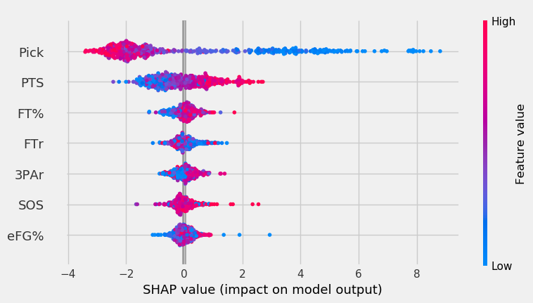
The graph below shows each feature’s impact on the SVM’s model output.
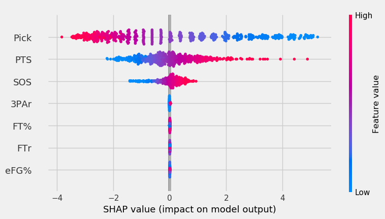
The color indicates the feature value, of the value we’re inputting. So, a point where the pick is blue indicates that the player was picked early. The x-axis shows the impact on model output. The features are sorted vertically by importance (top = most important feature, bottom = least important).
For the SVM, low pick values had a very high impact on model output. PPG was the second most important feature. High PPG impacted the output positively much more than low PPG impacted the output negatively. Lastly, SOS had the third highest importance.
The rest of the features had minimal importance. This is partially because the model explainer for the SVM had to be based off a sample of the data instead of the entire thing, like the RF and XGB. The KNN also had this issue. The RF and XGB will show more sensitivity to the other features.
The graph below shows the RF’s feature impact.
Yet again, pick was by far the most important feature, with PPG coming in second. Though SOS had the second lowest feature importance, the red points on the right show that very high SOS values had more impact on the model’s output than FT%, FTr, or 3PAr. The same goes for eFG%. Though it had the smallest impact on the model, when there was a very low eFG% value, it affected the model more than other features. Interestingly, it seems that lower FTr had a more positive impact on output – this is the opposite of what we’d expect.
The graph below shows the KNN’s feature impact.
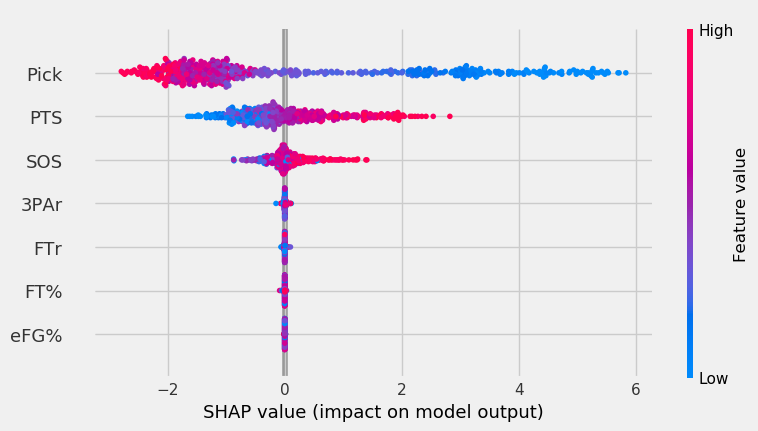
Like the other models, pick and PPG were the most important features. SOS came in third, and, like the SVM, other features had minimal impact.
The graph below shows the XGB’s feature impact.
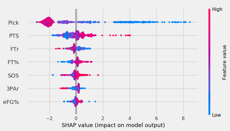
After pick and PPG, FTr was the most important feature. Surprisingly, as it did in the RF, lower FTr positively affected output. Though SOS was the third least important feature, its highest values impacted the model more than features like FTr and FT%.
In each of the four models, the spot at which the player was picked was the most important feature followed by PPG. Each model had eFG% as its least important feature.
Conclusion
Though the models had low r-squared values, they passed the standardized residuals test and performed accurately last year. Each model predicts Zion will have the highest PPG. The RF and XGB like Ja Morant as the second highest scorer, while the SVM and KNN predict R.J. Barrett will be the second highest.
Past the top three, all the models are higher on the first two point guards off the board – Darius Garland and Coby White – than they are on forwards in the range like Deandre Hunter and Cam Reddish.
Later in the first round, the models like Bol Bol and Carsen Edwards. Bol Bol has the biggest difference between the Ringer’s ranking and his average projected PPG ranking. While the Ringer ranks him 19th, he had the 10th highest projected PPG. Edwards had the second highest jump; despite his ranking of 26th, the models project he will have the 19th highest PPG.
The biggest fallers between the Ringer’s ranking and projected PPG were Nicolas Claxton (16th overall vs. 23rd highest PPG) and Matisse Thybulle (21st overall vs. 27th highest PPG). This is expected given that both project to be excellent defenders with questionable offensive games.
The table below shows each model’s predicted PPG, the Ringer’s ranking of the player, and the average predicted PPG.
| Ringer mock draft rank (NCAA) | Player | SVM | RF | KNN | XGB | Average |
|---|---|---|---|---|---|---|
| 1 | Zion Williamson | 15.2 | 16.2 | 15.3 | 15.8 | 15.6 |
| 2 | Ja Morant | 10.9 | 14.9 | 10.9 | 13.2 | 12.5 |
| 3 | R.J. Barrett | 14.2 | 12.7 | 14.1 | 12.5 | 13.4 |
| 4 | Jarrett Culver | 10.5 | 12.2 | 11.0 | 11.4 | 11.3 |
| 5 | Deandre Hunter | 9.2 | 7.5 | 9.0 | 9.3 | 8.7 |
| 6 | Darius Garland | 9.7 | 12.7 | 9.2 | 12.9 | 11.1 |
| 7 | Coby White | 9.8 | 12.4 | 10.1 | 10.1 | 10.6 |
| 8 | Cam Reddish | 8.7 | 9.8 | 8.7 | 7.9 | 8.8 |
| 9 | Jaxson Hayes | 7.1 | 6.9 | 7.0 | 6.9 | 7.0 |
| 10 | Brandon Clarke | 6.7 | 5.9 | 6.9 | 5.0 | 6.1 |
| 11 | Rui Hachimura | 5.8 | 6.4 | 5.5 | 5.6 | 5.8 |
| 12 | Nassir Little | 6.0 | 5.3 | 6.2 | 5.3 | 5.7 |
| 13 | Nickeil Alexander-Walker | 6.0 | 4.9 | 5.5 | 6.5 | 5.7 |
| 14 | Romeo Langford | 7.0 | 6.5 | 5.7 | 5.9 | 6.3 |
| 15 | Keldon Johnson | 5.9 | 6.5 | 5.7 | 5.7 | 5.9 |
| 16 | Nicolas Claxton | 4.0 | 3.7 | 5.3 | 4.2 | 4.3 |
| 17 | Tyler Herro | 5.5 | 5.6 | 5.0 | 5.9 | 5.5 |
| 18 | P.J. Washington | 4.9 | 6.7 | 6.0 | 5.0 | 5.6 |
| 19 | Bol Bol | 6.2 | 7.2 | 6.0 | 6.4 | 6.4 |
| 20 | Ty Jerome | 3.7 | 5.2 | 4.5 | 3.2 | 4.1 |
| 21 | Matisse Thybulle | 3.0 | 4.3 | 4.3 | 4.4 | 4.0 |
| 22 | Cameron Johnson | 3.7 | 5.5 | 4.6 | 4.3 | 4.5 |
| 23 | Grant Williams | 4.5 | 4.7 | 5.2 | 4.8 | 4.8 |
| 24 | Kevin Porter | 2.5 | 4.8 | 3.4 | 4.3 | 3.7 |
| 25 | Talen Horton-Tucker | 3.3 | 4.3 | 4.4 | 4.3 | 4.1 |
| 26 | Carsen Edwards | 4.5 | 5.3 | 4.9 | 4.9 | 4.9 |
| 27 | Dylan Windler | 2.4 | 5.2 | 4.8 | 5.2 | 4.4 |
| 28 | Mfiondu Kabengele | 2.8 | 5.0 | 4.1 | 4.5 | 4.1 |