Summary of average predicted PPG:
Introduction
The differences between college and NBA basketball make it difficult to predict shooters’ ability or PPG in traditional ways. College basketball has not only a shorter three-point line, but also vastly different defenses than the NBA. Therefore, attempting to predict a prospect’s shooting ability using just their college 3PT% provides inconsistent results. This has lead scouts to examine other stats to predict a player’s shooting ability, such as FT%.
By now, most scouts have accepted that FT% is probably a better indicator of a good shooter than 3PT%. This assumption is made because free throws demonstrate a prospect’s pure form; so, aside from a few exceptions, a great free throw shooter will have sound fundamentals.
Last year’s draft presents this classic dilemma. Though it’s far too early to say that Markell Fultz and Lonzo Ball will not be good shooters, as of now, they are significantly worse shooters than Jayson Tatum. However, Ball and Fultz both had significantly higher 3PT% than Tatum. Fultz and Ball shot 41.3% and 41.2% from 3, respectively, compared to Tatum’s 34.2%. However, this year, Tatum shot 43.4% from 3, compared to Fultz and Ball’s 0% (0 for 1) and 30.5%, respectively.
These large differences show how difficult it is to accurately predict a prospect’s shooting ability. However, using several shooting factors as inputs in a machine learning model to predict PPG gives more accurate results, as all shooting factors are considered. With a machine learning model that accounts for all these inputs, we can try to predict the top shooters by PPG in this upcoming draft.
Methods
First, I gathered college and NBA shooting data of players who met the following criteria:
- Drafted starting with the 2013 draft
- Average at least 1 3PM/G in their career
- Played at least half of the games they could have played since being drafted
- Played in college
The 2013 draft limitation was established so that all the players played only in the modern NBA for their whole career. The 1 3PM/G limitation was established because the NBA’s minimum 3PM to be considered in league-wide 3PT% is 82, or 1 per game. The players must have played in college and not internationally so that the context is more similar, thereby making the comparison more accurate.
47 players met all these restrictions. For these players, the following stats about their college and NBA careers were recorded:
| College | NBA |
|---|---|
| FG% | FG% |
| 2P% | 2P% |
| 3P% | 3P% |
| FT% | FT% |
| TS% | TS% |
| eFG% | eFG% |
| 3PAr | PTS/G |
| FTr |
Then, I recorded the same data for this upcoming draft class. My restrictions were:
- Must be in the first round of The Ringer’s 2018 NBA Draft Guide (as of 5/21 update)
- Must have at least 1 3PM/G in college career
The machine learning model was then created using scikit-learn. The following three models were created, all of which had a test size of 0.20 (20% of the data was used as the validation set):
- Linear regression
- Ridge regression
- Support vector regression
After these models were created and their accuracy was tested, this year’s draft class was put into each of the models. When the draft class data is put into each model, the model predicts the points per game for each player. Though the model predicts PPG, it is important to note that the model essentially predicts the PPG for each player assuming their conditions in the NBA are the same. Clearly, a top-5 pick on a tanking team will get more shot opportunities and minutes (and therefore points) than a late pick on a contending team. However, the model can’t adjust for this, because we don’t know each player’s situation. So, the model really predicts an “all else equal” PPG for each player.
The natural issue with the analysis
Aside from the fact that the models are not perfectly accurate (as expected), there is an innate issue with the model: the data is skewed. Only NBA players who played at least half of the games they could have played since being draft and players who have at least 1 3PM/G were used to create the model.
This makes the data problematic, as creating these restrictions make each player in the model a successful NBA player. So, the draft class is only being compared to successful NBA players; this will raise their expected PPG and make the range of predicted PPG much narrower, as all the players are being compared to good NBA players.
For example, there might be several players who have the exact same college stats as many of the players in this draft class, but turned out to be complete busts. If they busted, they would have either not played have of their possible games or have at least 1 3PM/G in their career.
Therefore, the model is skewed. However, the model can still give a good estimate of PPG even if only successful players are used. This is evident in the fact that the regressions show results that we would (mostly) expect; the last pick in the first round in The Ringer’s mock draft did not have the highest predicted PPG, and with the exception of Trae Young in the support vector regression, the top picks in the draft had the highest predicted PPG.
Despite its deficiencies, the model is still better than simply predicting an NBA statistic using one college statistics. For example, notice how poorly college 3PT% and PPG predicted NBA 3PT% and PPG:
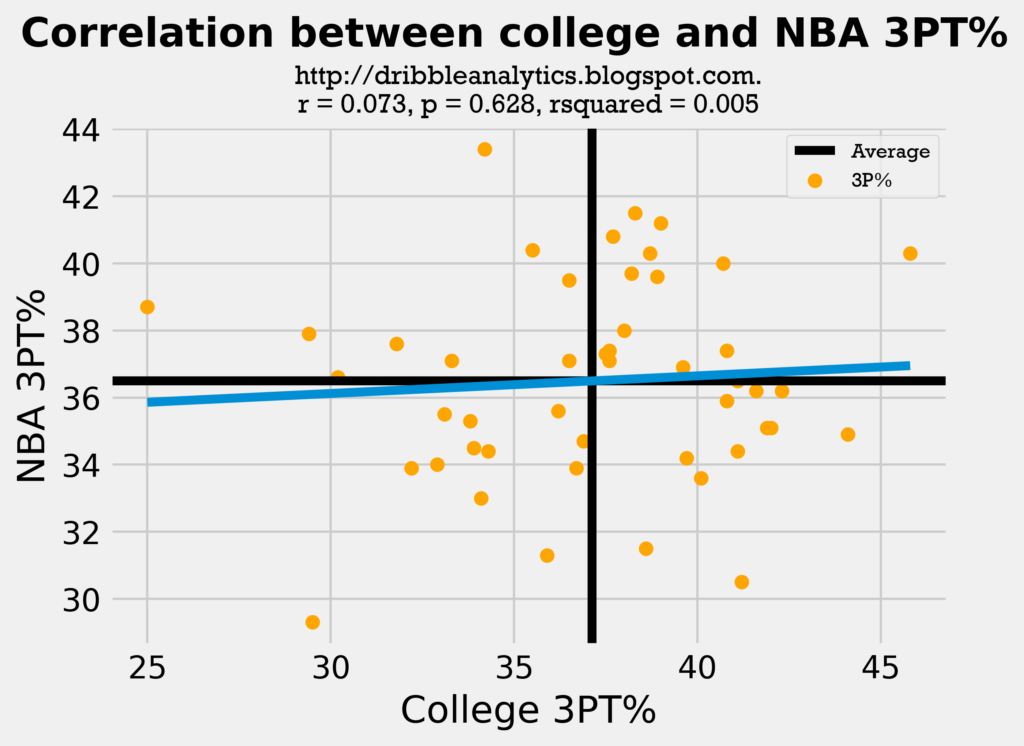
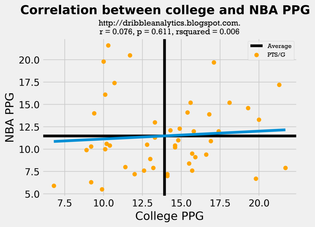
An r-value, or correlation coefficient, of 0 implies that there is no correlation between the two factors. These two regression had an r-value of almost 0, demonstrating that college 3PT% and PPG are almost fully uncorrelated to NBA 3PT% and PPG. Both regressions were also statistically insignificant, as they had p-value > 0.05. Both also had a very low r-squared, or variance score, demonstrating that the model fails to account for variance.
Because of the problems with these more simple ways to predict NBA stats when given college stats, I feel the machine learning model can provide a good estimate of NBA PPG. Even though the data is skewed by naturally removing busts, the model still has significantly higher accuracy than the two above regressions.
Comparing college and NBA stats
Because the two regression models above were very poor, it’s important to see that our players had similar stats in college and the NBA. Comparing these similarities will let us evaluate whether it’s worth making a model at all, or if the stats or significantly different. We can then compare the past players’ data to the draft class’s data to see if their college stats were similar to the past players’ college stats. If they are similar, then it means it’s mostly reasonable to create a model to predict this draft class’s PPG using previous players’ college stats.
To look at the similarity between these stats, we’ll look at histograms at 3PT%, FT%, and PPG of the past players’ in both college and the NBA. We’ll also look at histograms of these same statistics for this draft class. If the mean and standard deviation is close between all the histograms, and the range is not drastically different, then we can expect the machine learning model to be consistent (and therefore, reasonable to make).
Below are the histograms of the past players’ 3PT% in collge and the NBA, followed by a histogram of the draft class dataset’s 3PT%:
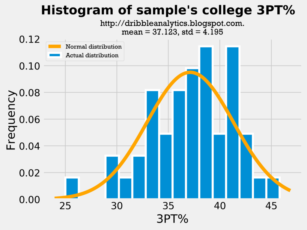
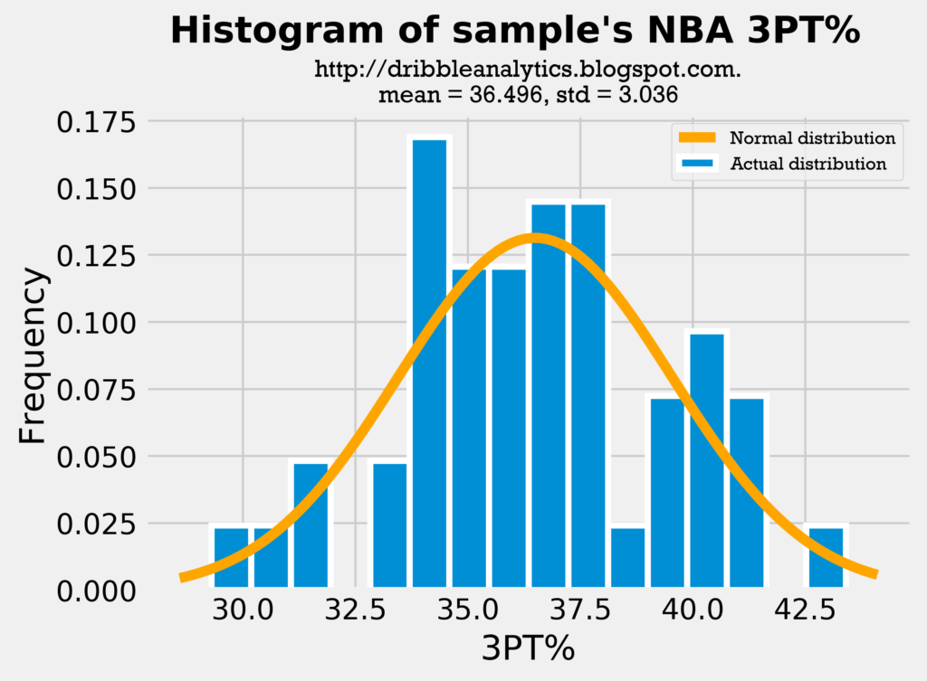
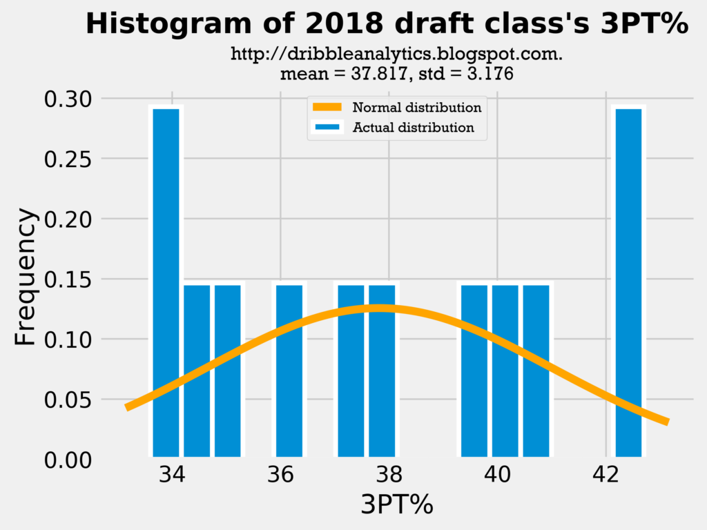
Because both the mean and standard deviation in all the histograms are close, it is fair to use college 3PT% as a predictor of shooting, given that it does not change too much once players enter the NBA. Because the draft class’s mean 3PT% and standard deviation of 3PT% is close to the sample’s, we can make the comparison between them. Let’s see if the same applies to their PPG:
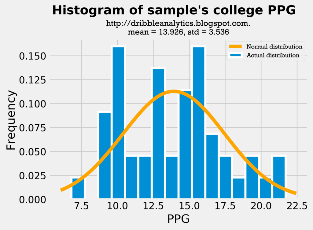
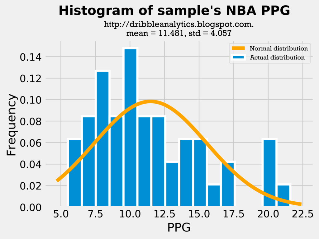
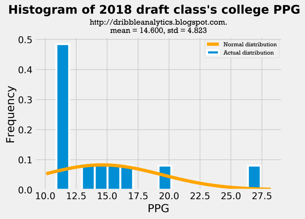
Though the difference here is much larger than in 3PT%, this difference is expected. Because most of the sample’s players were drafted in the first round, they likely played big roles on their college teams. So, we would expect their college PPG to be higher than their NBA PPG. The important comparison here to test the fairness of including PPG in the analysis is between the sample’s college PPG and the draft class’s PPG. The mean and standard deviation of these datasets are close, making the analysis reasonable.
Below are histograms of the players’ FT%. This is the final metric I’ll examine with histograms, because if these three metrics are close, then all the other metrics (FG%, eFG%, etc.) are also probably close.
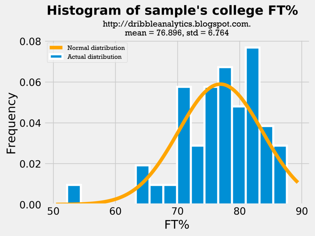
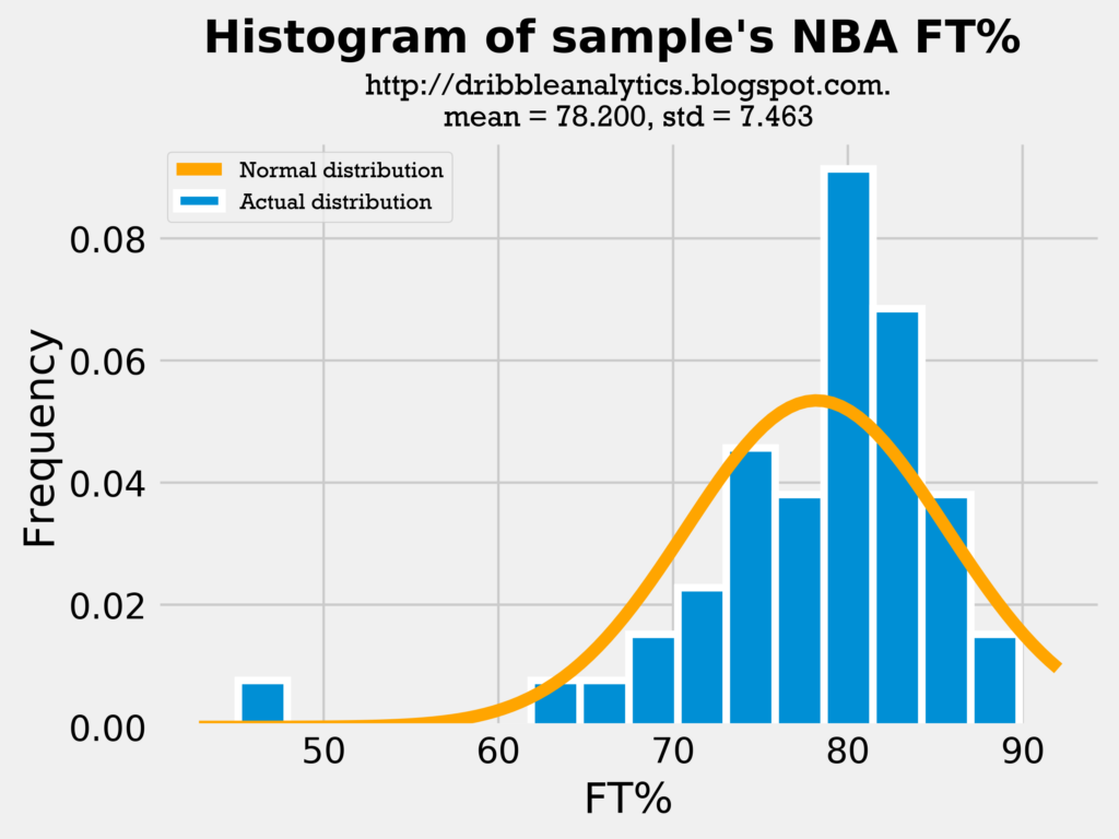
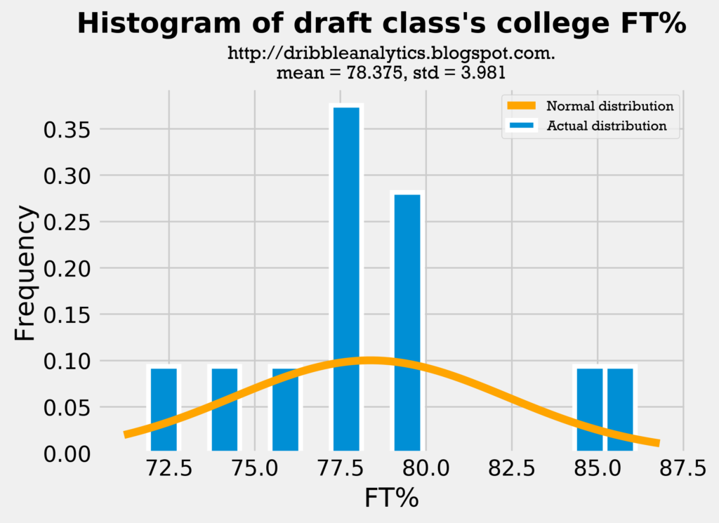
All three histograms show the mean FT% is close. Though the draft class’s standard deviation is much lower than the sample’s, this may actually be a good sign, as lower variance will make the model more accurate.
Because all three measures demonstrated similar means and standard deviations, the comparison between the draft class’s data and sample’s data (both in college and in the NBA) is reasonable.
Model results
Once I gathered all the data, I made the model by using scikit-learn’s train test split function. I made the test set 20% of the dataset. This means that 20% of the sample player dataset was used to test the model’s accuracy and determine the coefficients of correlation, while 80% of the sample player dataset was used to teach the model.
With the train test split function, the inputs were all of the metrics measured for college players (FG%, 2P%, 3P%, FT%, TS%, eFG%, 3PAr, FTr, and PTS/G). All these metrics were used to create one output: NBA PTS/G. Three different types of regressions were used:
- Linear regression
- Ridge regression
- Support vector regression
Regression explanations
A linear regression models input variables and outputs to create a line. They are often made using the “least squares” method, where the line is created such that the squared distance between the line’s predicted outcome and the real data point is minimized. A ridge regression models input variables to output variables by creating a vector x so that the input vector, A, multiplied by x, equals the output vector B.
A support vector regression is an extension of the support vector machine, which is a form of supervised learning.
Regression accuracy
The two graphs below demonstrate the accuracy of the three regressions. The most accurate regression will have the highest r-squared and the lowest mean squared error.
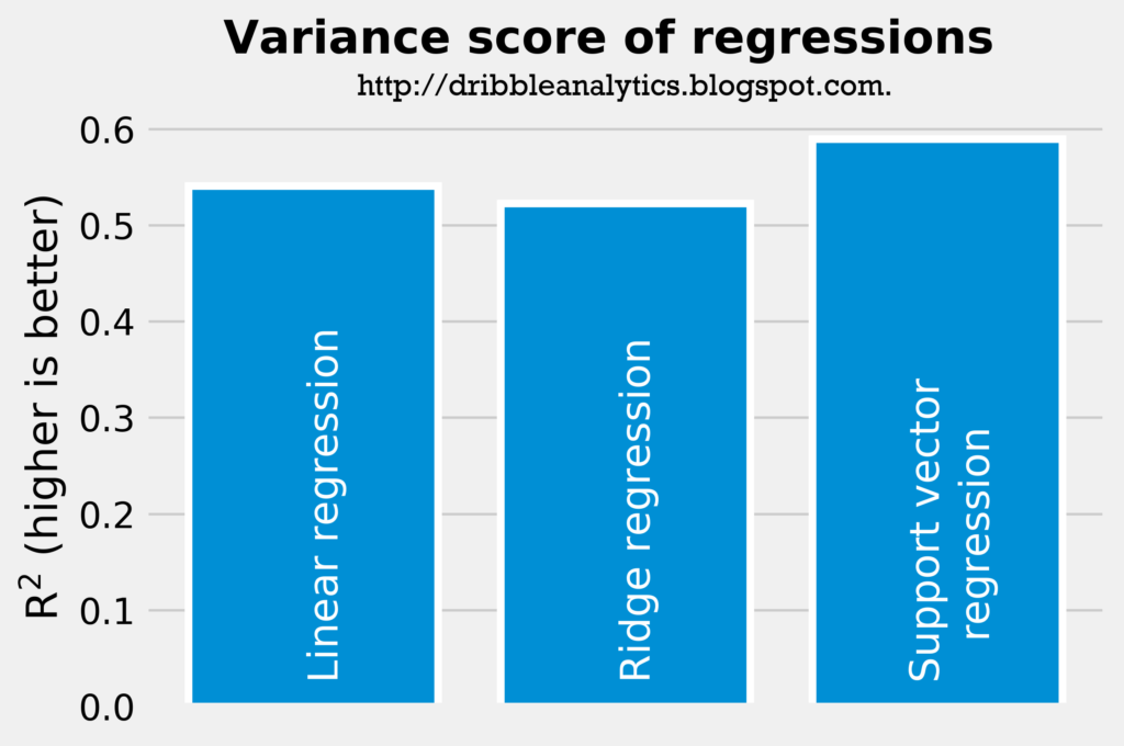
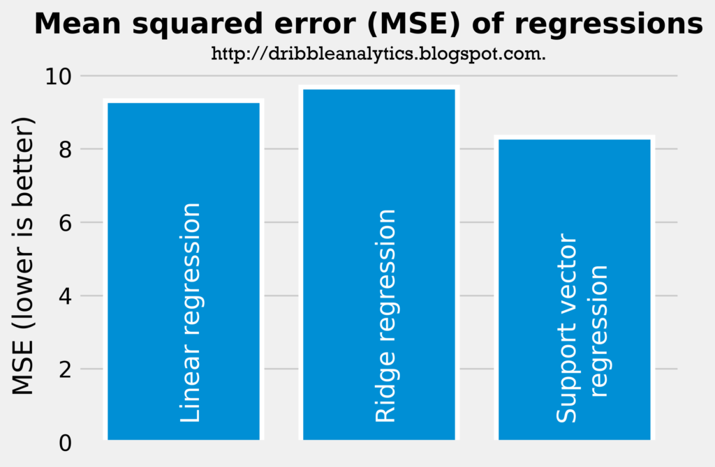
According to just the r-squared and mean squared error, the support vector regression is most accurate, followed by the linear regression and then the ridge regression. Nevertheless, the difference in accuracy between these models is not too big (the support vector regression has an r-squared of 0.590 compared to the ridge regression’s r-squared of 0.523). All the models seem accurate enough for us to consider their results.
Regression results
Note that though the models predict PPG, they can’t account for differences in playing time, team situation, or shots. Therefore, they predict an “all else equal” PPG. The graph below shows the predicted PPG of the draft class dataset using a linear regression:
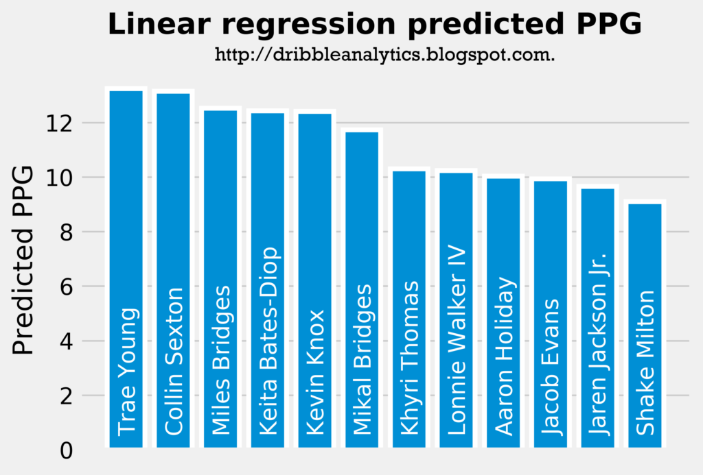
These results seem pretty reasonable, as the players at the top of the draft have a higher predicted PPG, as we would expect. The only major outlier here is Jaren Jackson Jr., but this is not too surprising given that he played on a strong Michigan State team and that a large part of his draft stock is his superb defense.
The graph below ranks the predicted PPG from the ridge regression:
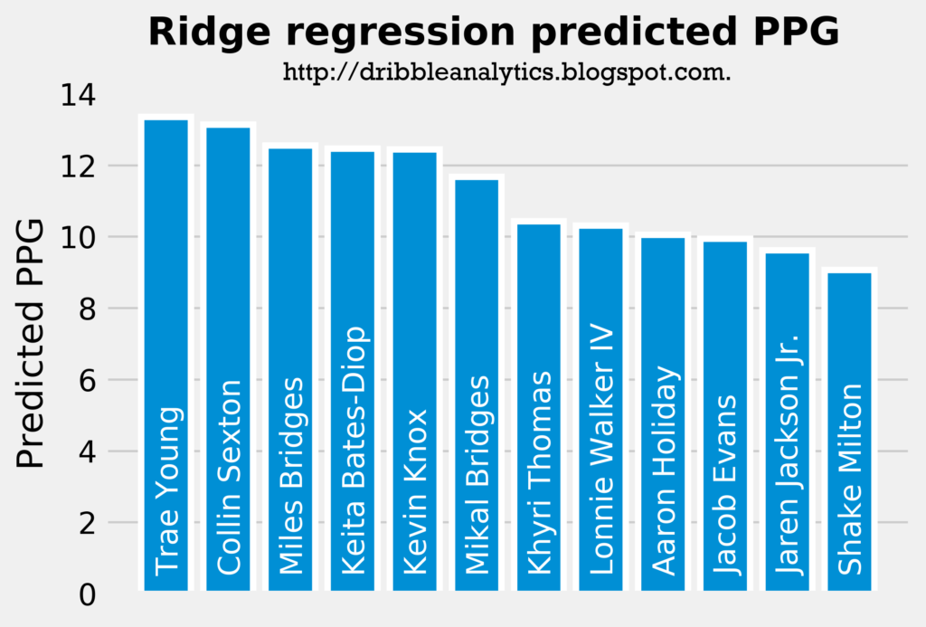
This regression gives the exact same ranking for PPG as the linear regression (the order of the best shooters is the same as the linear regression). However, it projects a bit more points for each player. Again, these results are not too surprising.
The graph below shows the support vector regression’s predicted PPG. Note that this is the most accurate regression of the three.
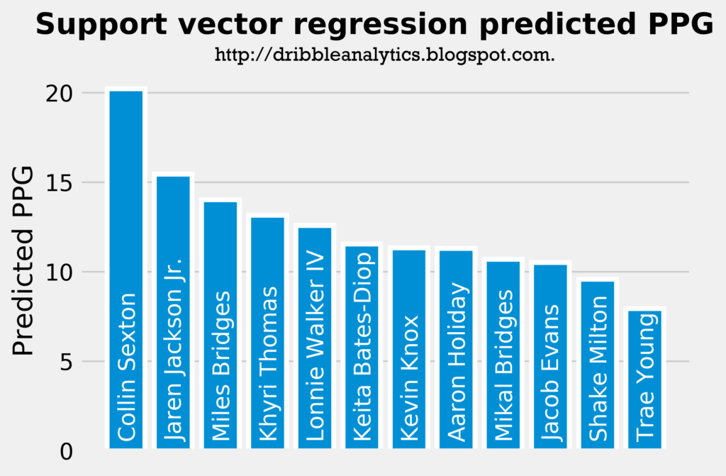
These results are surprising. The model predicts that Collin Sexton will be by far the best shooter in the draft class, and that Trae Young will be the worst. Furthermore, this is the only regression of the three to favor Jaren Jackson Jr. Lastly, it places some late first-round picks (Khyri Thomas, Lonnie Walker IV, and Keita Bates-Diop) over lottery picks like Kevin Knox and Mikal Bridges.
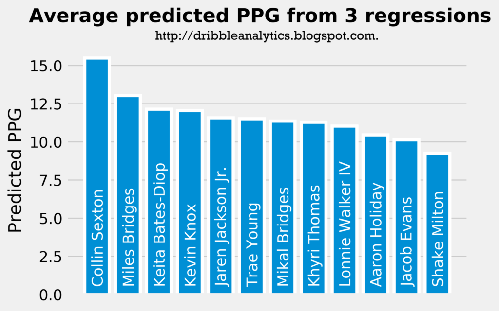
Lastly, let’s examine the average predicted PPG from all three models:

Interestingly, Collin Sexton has the highest predicted PPG. This is because he had the second highest PPG in the linear and ridge regressions, and had the highest PPG by a significant margin in the support vector regression. Trae Young places 6th because the support vector regression predicted the lowest PPG for him, even though he had the highest predicted PPG in the other two regressions.
Regression coefficients
Unfortunately, because the support vector regression does not use a linear kernel in scikit-learn, I can’t calculate regression coefficients for the support vector regression. However, coefficients can be calculated for the other two models. They are as follows:
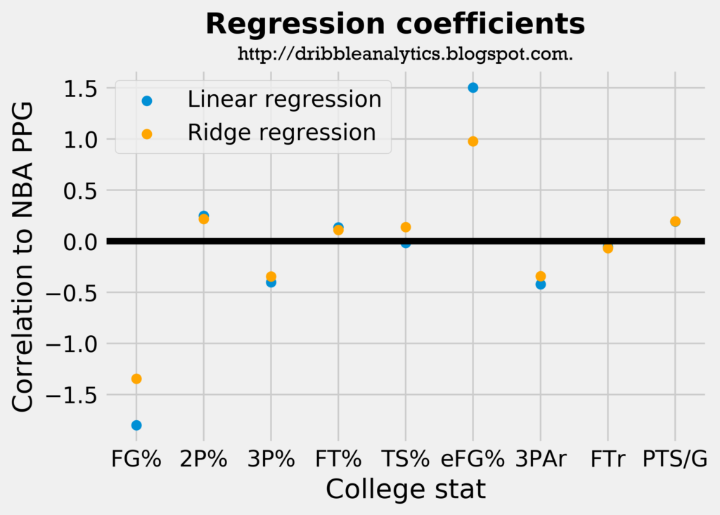
eFG% proved to be most correlated to PPG in these two models. Interestingly, FG% had a strong negative correlation to PPG, and 2P% had a higher coefficient than 3P% even though the datasets were restricted based on 3-point shooting.
Improving accuracy for future tests
For this analysis to be done more accurately, the biggest change would be to change the criteria for the sample player dataset. If the draft class dataset is selected by players who are in the first round of a mock draft and average at least 1 3PM/G, then for the most consistent results, the sample player dataset should consist of players drafted in the first round who averaged at least 1 3PM/G in college.
Not bad – certainly a tough analysis to do.
In addition to fitting regressions, you could also consider identifying "comparable college seasons" between players in the current draft (or next years draft), and current NBA players.
Who were the 25 players with the most similar ("similar" can be measured in different ways) college seasons to Collin Sexton? How many PPG did those 25 players average in their rookie and sophomore years?