Thanks to Reddit user SamShinkie for providing me with the historical database I used in this project.
Summary
Of the historical dataset, only 8.75% of players were all stars, and only 1.95% were hall of famers. Therefore, from the 2017 draft class sample of 30 players, we would expect 2-3 all stars and maybe 1 hall of famer. The models predict no hall of famers. All the models predict Ben Simmons will be an all star, and one of the models (the deep neural network) predicts Donovan Mitchell will be an all star.
Introduction
Following strong rookie years and playoff performances from Ben Simmons, Jayson Tatum, and Donovan Mitchell, many view all three players as future all stars. Furthermore, other rookies such as Lonzo Ball and Lauri Markkanen showed promise on lottery teams, giving fans hope they, too, could be all stars.
In many cases, a strong rookie year does not translate into ascension to all star-level. For example, some previous rookie of the year winners include Michael Carter-Williams, Tyreke Evans, and Andrew Wiggins. All three of these players had extremely promising rookie years; therefore, it is hard to pinpoint why several rookie of the year winners go on to become superstars while these players barely improved.
Because of this wide variety of outcomes, it is difficult to tell who will succeed from the 2017 draft class by simply comparing the rookies to each other. By using machine learning classification algorithms trained on every rookies season in the 3-point era, I attempt to sort 2017’s rookies into hall of famers and not-hall of famers, and all stars and not-all stars.
Methods
Using SamShinkie’s database of both counting and advanced stats for every player in NBA history, I retrieved the stats for every player’s rookie year in the 3-point era (1979-80 season). The database includes all the player’s stats available on Basketball Reference. I did not use all the stats in the database, as some can be linearly predicted from other stats (such as FG% from FG and FGA). This creates multicollinearity, which leads to high variance results from models that are often overfitting.
I used the following stats as inputs in the models:
| Shooting stats | Defensive/passing/rebounding stats | Other stats |
|---|---|---|
| FG/G | AST/G | G |
| FGA/G | STL/G | MPG |
| 2P% | BLK/G | |
| 3P% | TOV/G | |
| FT% | PF/G | |
| TS% | TRB/G | |
| 3PAr | ||
| FTr |
I made separate models to predict hall of famers and all stars. In both models, 1 is the positive result – meaning the player is predicted to be a hall of famer or all star – and 0 is negative – meaning the player is predicted to not be a hall of famer or all star.
Using lists of every NBA all star and hall of famer – excluding coach and GM hall of famers – from Basketball Reference and Hopphall, I assigned the 0 and 1 values to each player. Players with above a 90% hall of fame probability in Basketball Reference’s hall of fame probability calculator were also assigned a 1. Though Manu Ginobili has only a 20.05% hall of fame probability according to Basketball Reference, he was assigned a 1 given that it’s clear he will be a hall of famer.
I made four types of models:
- Support vector machine (in this case, a support vector classifier)
- Random forest
- k-Nearest Neighbors
- Deep neural network
Because I made separate models to predict hall of famers and all stars, 8 models in total were created. All models were created by using a train/test split with a test size of 25%.
After creating the models, I performed a randomized search on hyperparameters to see if the models’ can be more accurate with different parameter values. However, the randomized search proved to make no difference in the accuracy score, meaning that randomized hyperparameters did not make the models predict a 1 for a player they previously predicted a 0 (or the other way around). Because the randomized search did not improve model accuracy, I proceeded with the initial models.
The same stats in the above table were recorded for every player who played over 50 games in the 2017 draft class. The 50 game limit was set so there is a decent sample size for the player’s stats. This limit cuts off Markelle Fultz, so he is not included in this analysis. In total, 30 players met this restriction, so the sample size consisted of 30 players.
Understanding the data
In total, out of 2618 players drafted since the 1980 draft, 51 made the hall of fame and 229 made at least one all star team. Therefore, 1.95% players drafted since 1980 were hall of famers, and 8.95% were all stars.
It is important to note that positive results – instances where the player was a hall of famer or all star – in the dataset were extremely rare. This means that a model could have an almost perfect score in some classification metrics by simply predicting every player as 0, or not a hall of famer or all star. Because of this possibility, it is important to take into account what different classification metrics measure, and whether the models are actually better than saying “no one will be a hall of famer or all star.”
Where the models fall short
As discussed in the introduction, there have been several successful rookies who were out of the league within five years. Likewise, there have been several rookies who got almost no playing time their rookie year, and turned out to be hall of famers or all stars. Therefore, it’s important to remember that the models do not know any of the following things:
- Narrative (this is more of a problem with any all star-related predictions, as all star selections are often based on popularity)
- Playing on a tanking team (which would help a rookie put up empty stats)
- Coaching, injuries, off-court issues, trades, or any other major changes to a player’s rookie year situation
Given that the models know only of a player’s individual counting stats in his rookie year, the models are completely blind to the above factors. The models do not know of a player’s situation and how it changes.
Model analysis techniques
To discuss the accuracy of the different models, I used a few different factors.
First, I used a basic accuracy score (correct predictions / total predictions; ranges from 0 to 1 with 1 being the “best”). I then created a confusion matrix to visualize the models’ classifications. This tells us, for example, whether a model has a high accuracy score solely because it predicts all 0s. After examining the confusion matrix, I also cross-validated the accuracy score to check for overfitting and see if it predicts differently on a different split of the data.
Given the distribution of the dataset, accuracy score must be taken with a grain of salt. In addition to accuracy score, I used log loss and area under the ROC curve. Log loss measures the models’ performance when given probability values between 0 and 1 as inputs. A “perfect” model will have a log loss of 0. Because log loss incorporates the uncertainty of the prediction, it may give us more insight into the models’ accuracy.
The receiver operating characteristic curve (ROC curve) plots the true positive rate (TP / (TP + FN)) against the false positive rate (FP / (FP + TN)). The area under the ROC curve is the space between the x-axis and the ROC curve. A “perfect” model will have an area under the curve of 1.
Given that the models that have a very low false positive rate (as they can predict almost everyone as a 0) will have a low true positive rate, the area under the ROC curve can tell us more about the models’ accuracy.
Hall of fame model analysis
The hall of fame models can have very high accuracy scores by predicting all 0s, given that out of a random sample of about 640 players, 6-7 of them would be hall of famers. Even though the random sample happened to include 11 hall of famers, this holds true.
Because of the lopsidedness of the data, cross-validation of the accuracy score won’t be very useful, either. The point of cross-validation is to test the model on a different split of data, but if such a low percentage of the data is positive, then a model predicting all 0s will be similarly accurate.
The table below shows the four models’ accuracy scores, cross-validated accuracy scores, and the 95% confidence interval for these cross-validation scores.
| Model | Accuracy score | CV accuracy score | 95% confidence interval |
|---|---|---|---|
| SVC | 0.983 | 0.98 | +/- 0.00 |
| RF | 0.986 | 0.98 | +/- 0.00 |
| KNN | 0.982 | 0.98 | +/- 0.00 |
| DNN | 0.988 | 0.98 | +/- 0.00 |
As expected, all four models have very high accuracy scores and cross-validated accuracy scores. The +/- 0.00 confidence interval indicates that the models did not make any predictions differently when assigned to a different test set. To see which models – if any – correctly predicted hall of famers and which models only predicted 0s, let’s look at the confusion matrices.
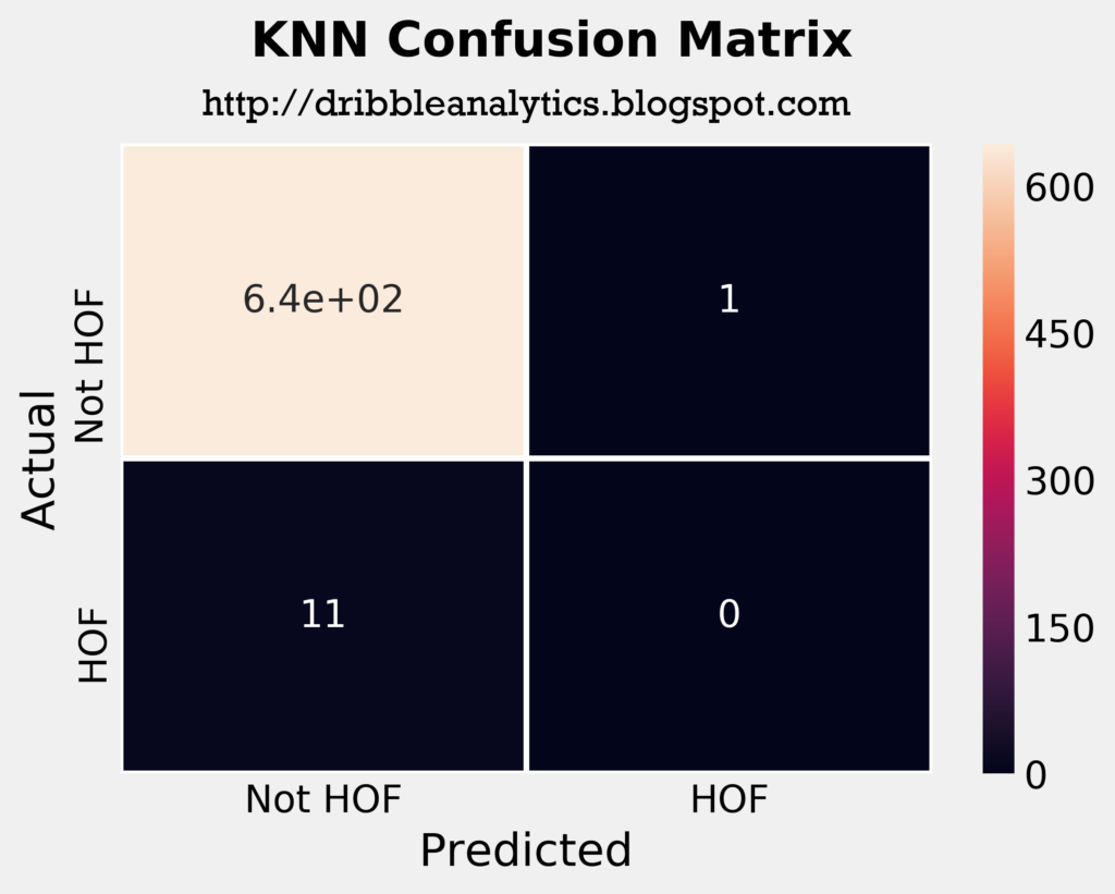
The four plots below are the confusion matrices for each of the four models.
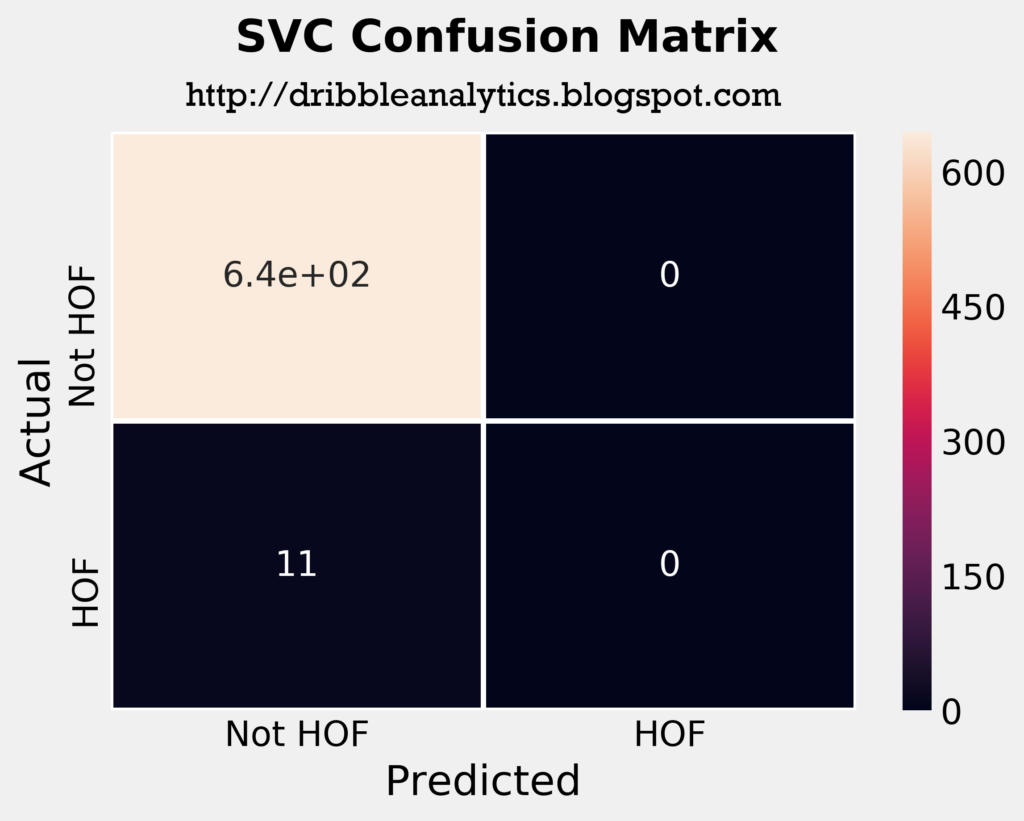


The confusion matrices tell us that the SVC predicted all players in the test set to not be hall of famers. So, just by looking at its confusion matrix and ignoring other metrics such as log loss and area under ROC curve, it’s not better than saying “no one will be a hall of famer.”
The RF correctly predicted 2 hall of famers, and the KNN incorrectly predicted one player as a hall of famer. The DNN had the most interesting results; it correctly predicted 5 players as hall of famers, and incorrectly predicted 2 players as hall of famers. This would make the DNN the most accurate model intuitively, ignoring all other metrics.
To get a deeper look at each model’s accuracy, let’s look at their log loss. Note that a lower log loss is “better”. The table below shows each model’s log loss.
| Model | Log loss |
|---|---|
| SVC | 0.066 |
| RF | 0.050 |
| KNN | 0.195 |
| DNN | 0.045 |
The log loss confirms the intuition that the DNN and RF are the most accurate models, given that they were the only two models to predict any hall of famers. The SVC is not far behind the RF, and the KNN has the highest log loss.
Now, let’s look at each model’s area under the ROC curve. The graph below plots each model’s ROC curve and calculates the area under each one.
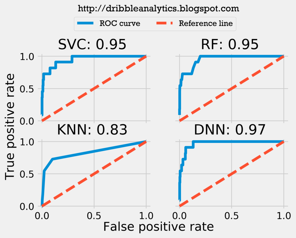
The ROC curve shows that the DNN is indeed the most accurate model, with the RF and SVC close behind. The KNN has the lowest area under the ROC curve by a decent margin.
Hall of fame model results
None of the four models predicted any of the rookies to be a hall of famer. This is not surprising given that only 51 out of 2618 players drafted since 1980 made the hall of fame. This rate of about 1.95% means that if each draft class had 30 players who I qualified for the model, there would be a hall of famer approximately every other draft class.
All star model analysis
Luckily, measuring the accuracy of the all star models will be more straightforward than the hall of fame models given that the all star models won’t get high accuracy scores by predicting all 0s.
The table below shows the 4 models’ accuracy scores, cross-validated accuracy scores, and 95% confidence interval for these cross-validation scores.
| Model | Accuracy score | CV accuracy score | 95% confidence interval |
|---|---|---|---|
| SVC | 0.927 | 0.92 | +/- 0.00 |
| RF | 0.933 | 0.92 | +/- 0.03 |
| KNN | 0.928 | 0.92 | +/- 0.01 |
| DNN | 0.930 | 0.93 | +/- 0.01 |
The models all have lower accuracy scores than the hall of fame models because of the greater number of all stars. Nevertheless, all four models have very high accuracy scores, and their performance remains constant when used on a different test set split.
The four plots below are the confusion matrices for each of the four models.
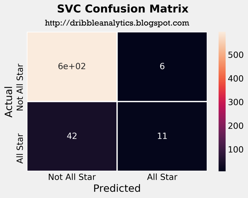

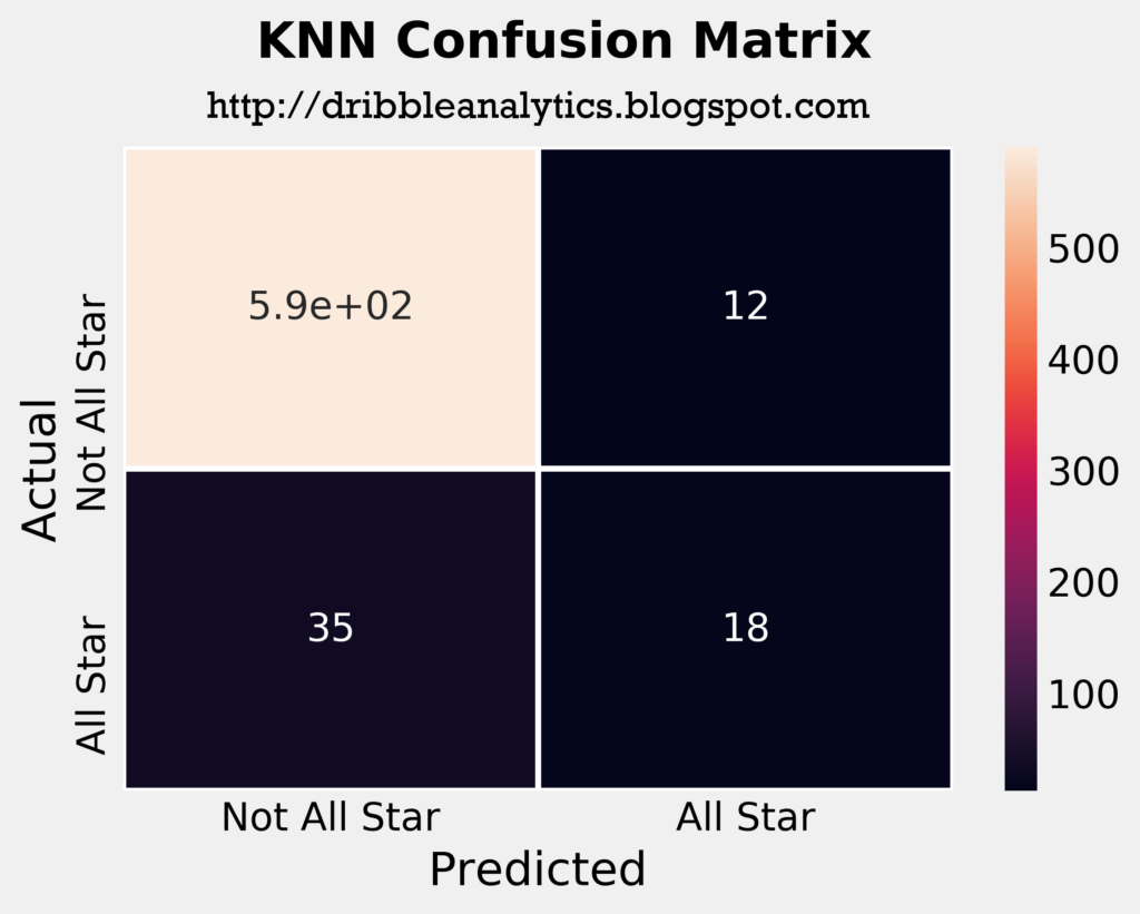

From a quick look at the confusion matrices, the RF seems to be the most accurate model. It correctly predicted the highest number of all stars out of the four models, and in consequence had the lowest number of incorrect “not all star” predictions.
The table below shows each model’s log loss.
| Model | Log loss |
|---|---|
| SVC | 0.231 |
| RF | 0.406 |
| KNN | 1.083 |
| DNN | 0.208 |
The log loss challenges our intuition that the RF is the most accurate model. The higher log loss for the RF indicates that there is more uncertainty in its predictions than in the SVC and DNN’s predictions. The KNN has a significantly higher log loss than the other three models, indicating it is likely significantly less accurate.
The graph below plots each model’s ROC curve and calculates the area under each one.
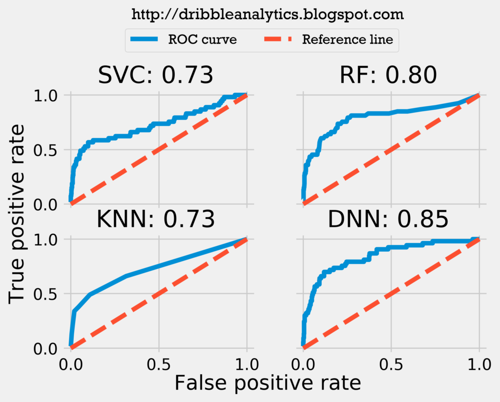
Both the log loss and ROC curve indicate the DNN is the strongest model. The ROC curve challenges the idea presented by the log loss that the SVC is the second most accurate model; instead, it suggests the RF is the second most accurate by a decent margin.
All star model results
All four models predicted Ben Simmons will be an all star. The DNN – seemingly the most accurate model by our tests – also predicted Donovan Mitchell will be an all star. No one else was predicted to be an all star by any model.
Conclusion
Though many of last year’s rookies seem very promising, it is unlikely more than a couple turn out to be all stars or hall of famers given a historical look at the data since 1980. The percentage of players since the 1980 draft who were hall of famers and all stars indicates that 1 in every 51 players will be a hall of famer (so 1 in every 2 samples of 30) and 1 in every ~11 players will be an all star (so 2-3 in a sample size of 30).
This distribution’s application to 2017’s draft class is supported by the models; there were no predicted hall of famers, and only 2 predicted all stars out of a sample of 30. All four models predicted Ben Simmons will be an all star, and the DNN predicted Donovan Mitchell will be an all star.