Summary
The average of the models show Chris Paul should have won over Kobe Bryant in 2008. LeBron over Rose in 2011. Harden over Westbrook in 2017.
Introduction
In the past 10 years, there have been multiple controversial MVP picks. Most recently, many debated whether Westbrook should have won over Harden in 2017. On the one hand, Westbrook had more points and rebounds, and also averaged a triple double for the year. On the other hand, Harden had more assists and higher efficiency, while also leading the Rockets to the third seed in the West, compared to the Thunder’s six seed.
Westbrook’s sparked a debate that still lasts today. Many discuss whether he is deserving of his MVP, given that no other MVP winner was on a team lower than the third seed. Though Harden ended up getting his MVP this year, many believe he should have won over Westbrook.
To determine who should have won this MVP race, along with other previous controversial MVPs such as Kobe over Paul in 08, Rose over Lebron in 11, Curry over Harden in 15, I created various models to analyze who should have won MVP the past 10 years given almost 40 years of previous MVP data.
Methods
First, I created a database of all the players who were top 10 in MVP votes since 1979-1980 (the season when the 3 point line was introduced). For these players, I measured the following stats:
| Counting stats | Advanced stats | MVP votes | Team stats |
|---|---|---|---|
| G | WS | MVP votes won | Wins |
| MPG | WS/48 | Maximum MVP votes | Overall seed |
| PTS/G | VORP | Share of MVP votes* | |
| TRB/G | BPM | ||
| AST/G | |||
| STL/G | |||
| BLK/G | |||
| FG% | |||
| 3P% | |||
| FT% |
* Vote share = % of maximum votes – adding together every player’s vote share does not equal 1. The only player with a vote share of 1 is Steph Curry in the 2015-2016 season, when he was the unanimous MVP.
Win shares, VORP, and team wins were scaled up to an 82 game season in the lockout years of 1998-1999 and 2011-2012.
Using all the counting stats, advanced stats, and team stats listed above – with the exception of WS/48 – I created four models to predict a player’s vote share. WS/48 was excluded because it can be linearly predicted by MPG, G, and WS. Vote share was used as the output because the maximum number of MVP votes increased over time, so MVP votes won increased too.
With these inputs and outputs, I created four models:
- Support vector regression (SVM)
- Random forest regression (RF)
- k-nearest neighbors regression (KNN)
- Deep neural network (DNN)
The models were trained and tested on MVP data from 1979-2007, and then made predictions for the last decade of MVPs (2008-2018).
Where the models fall short
MVP is a subjective award. A player with better all around stats may lose the MVP to a player with worse stats because of factors such as narrative. Therefore, because the models take only objective stats in account to predict a subjective award, they cannot account for several factors. These include:
- Narrative
- Voter fatigue (the idea that journalists will not want to award LeBron 5 straight MVPs, so they get “tired” of voting for him and vote for someone else even if he had a better season)
- Triple doubles and players breaking records. To the models, the difference between Westbrook 10.4 assists and 10.7 rebounds and Westbrook averaging 9.9 assists and 9.9 rebounds is just a 0.5 assist and 0.8 rebound difference. So, it can’t account for the uniqueness of him averaging a triple double.
- Name value or popularity of a player
Basic predictors of MVP share
While I was collecting the data, I noticed that there were a few common themes among the MVP winners. Notably, they were often among the top scorers of the year, lead their teams to among the highest win totals, and had among the highest VORP and BPM. This is what most would expect as the basic factors in predicting an MVP, given that a player who scores lots of points is – usually – valuable. If the player who scores a lot of points also contributes to the game in other ways, his team will likely be among the best, and he will likely score highly in advanced stats measuring impact.
First, let’s look at the correlation between wins and MVP share.
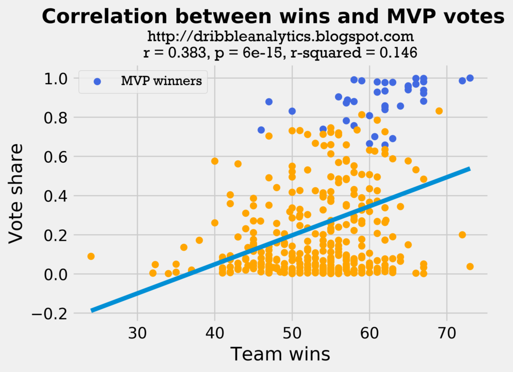
Most of the MVP winners seem to have very high win totals. The players who have very high win totals but low MVP shares are often supporting players to an MVP. For example, notice how at the two highest win totals (72 and 73 wins), there is an MVP (MJ and Curry) and then a supporting player with a low vote share (Pippen and Draymond).
The graph below shows the correlation between PTS/G and MVP vote share.
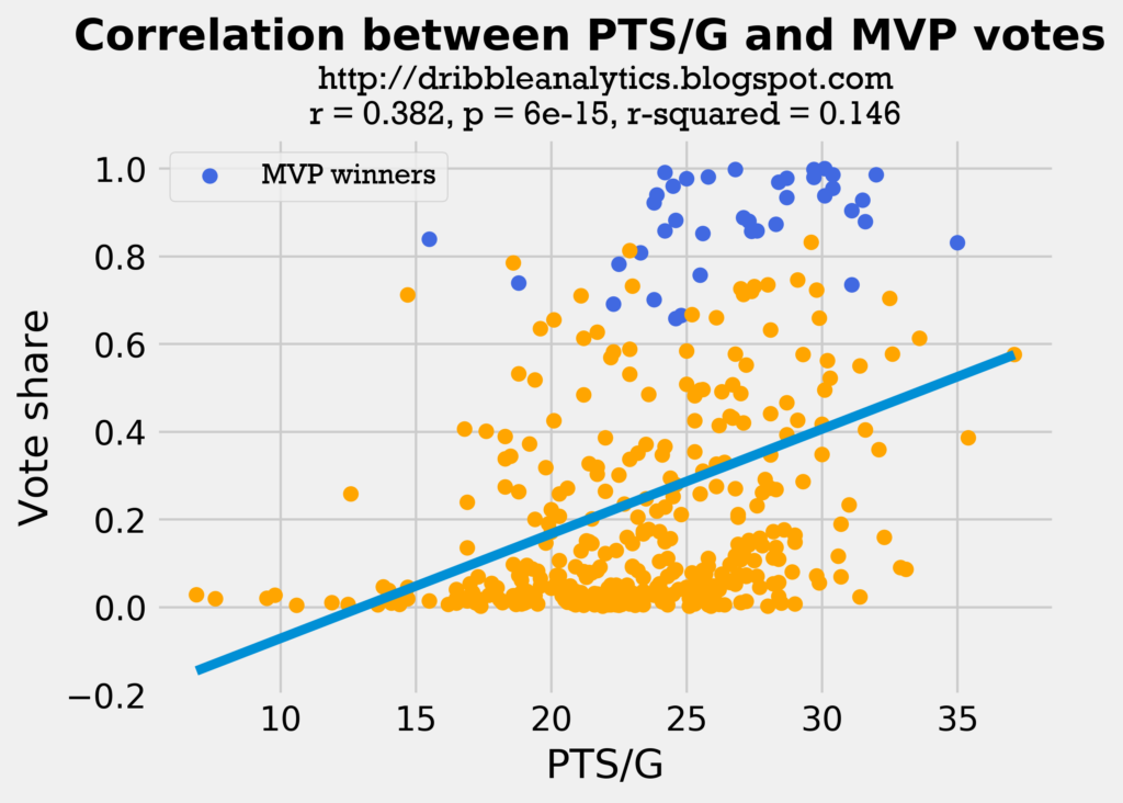
Interestingly, this correlation has an almost identical correlation coefficient (r-value) to the wins correlation. Additionally, if we look at the highest scorers in the dataset, only one has an MVP (MJ’s 1987-1988 season). This may be because players who have to carry such a large scoring load likely are not on good teams, and therefore do not win MVPs because their teams don’t win enough games.
The two graphs below show the correlations of VORP and BPM to MVP vote share.
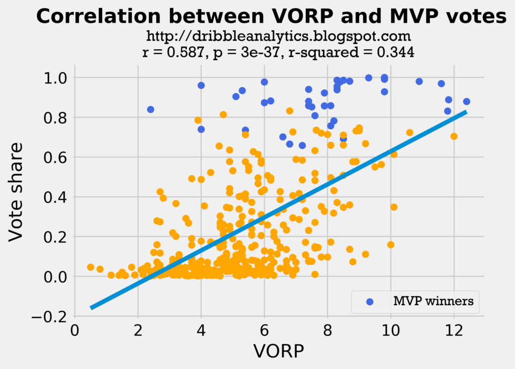
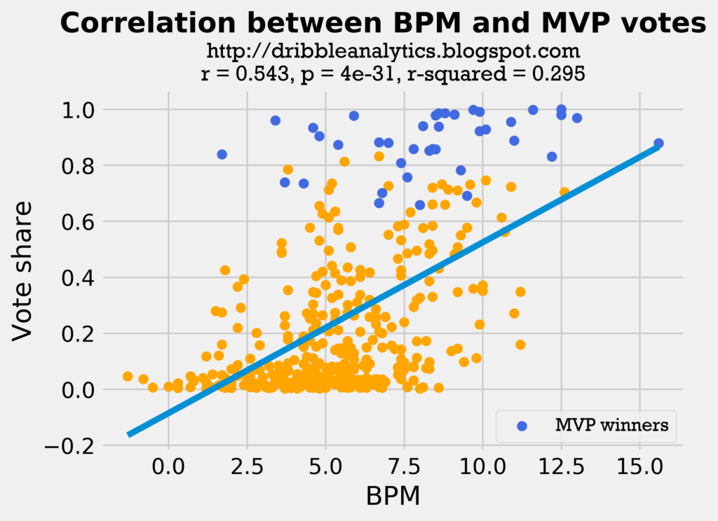
Both these regressions have higher correlation coefficients than the wins and PTS/G regressions. This is probably because though VORP and BPM measure individual impact, players on better teams have higher VORP and BPM. So, in a way, we could say that the VORP and BPM regressions take parts from combine both the wins and the PTS/G.
This gives us some hope that the models can have good accuracy by combining all the factors together.
Regression analysis
Basic goodness-of-fit and cross-validation
The table below shows the r-squared and mean squared error of the four models. Note that a higher r-squared is better, but that a lower mean squared error is better.
| Model | r-squared | Mean squared error |
|---|---|---|
| SVM | 0.669 | 0.028 |
| RF | 0.618 | 0.032 |
| KNN | 0.612 | 0.032 |
| DNN | 0.649 | 0.029 |
The models’ r-squared is not very good. Though it’s much higher than the r-squared of the simple regressions, it’s not very high to the point that it can be considered a very strong model.
However, the mean squared error shows that the models are very accurate despite their mediocre r-squared. The highest mean squared error and the models is 0.032. The smallest difference in vote share between first and second place among the entire dataset was 0.024. In most cases, it was significantly above 0.1. Therefore, this low mean squared error demonstrates that it predicted most – if not all – of the MVP winners correctly.
To examine if the models are overfitting, I perform k-fold cross-validation for r-squared with k = 3. If the models are overfitting, then the cross-validation r-squared will be significantly lower than the model’s r-squared. The table below shows the cross-validation score for r-squared and 95% confidence interval for the models from k-fold cross-validation.
| Model | CV r-squared | 95% confidence interval |
|---|---|---|
| SVM | 0.50 | +/- 0.25 |
| RF | 0.51 | +/- 0.20 |
| KNN | 0.42 | +/- 0.21 |
| DNN | 0.36 | +/- 0.38 |
All the models’ cross-validation score for r-squared is slightly lower than the measured r-squared. However, the r-squared for all models is within the 95% confidence interval for the cross-validation’s r-squared. Therefore, it is unlikely the models are overfitting.
Standardized residuals test
To further test the models’ accuracy, I performed a standardized residuals test. If the models have 95% of their standardized residuals within 2 standard deviations of the mean, and there is no noticeable trend in the residuals, then the model passes the standardized residuals test. Passing the standardized residuals test gives us a first indication that the models’ errors are random.
The graph below shows the standardized residuals of all four models.
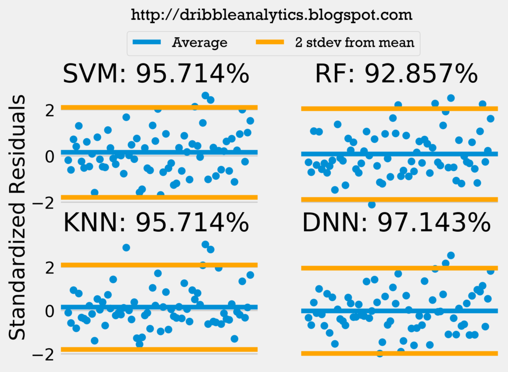
Only the random forest fails to pass the standardized residuals test. Because the random forest failed the standardized residuals test, we question whether its errors are truly random.
Q-Q plot
Another important consideration in a model’s accuracy is whether its residuals are normally distributed. To help visualize whether the residuals are normally distributed, I created a Q-Q plot (quantile-quantile). A Q-Q plot plots the quantiles of the residuals against that of a normal distribution. Therefore, normally distributed data will have a line of y = x with all the data points on or very close to that line.
The graph below shows the Q-Q plot of the models’ residuals.
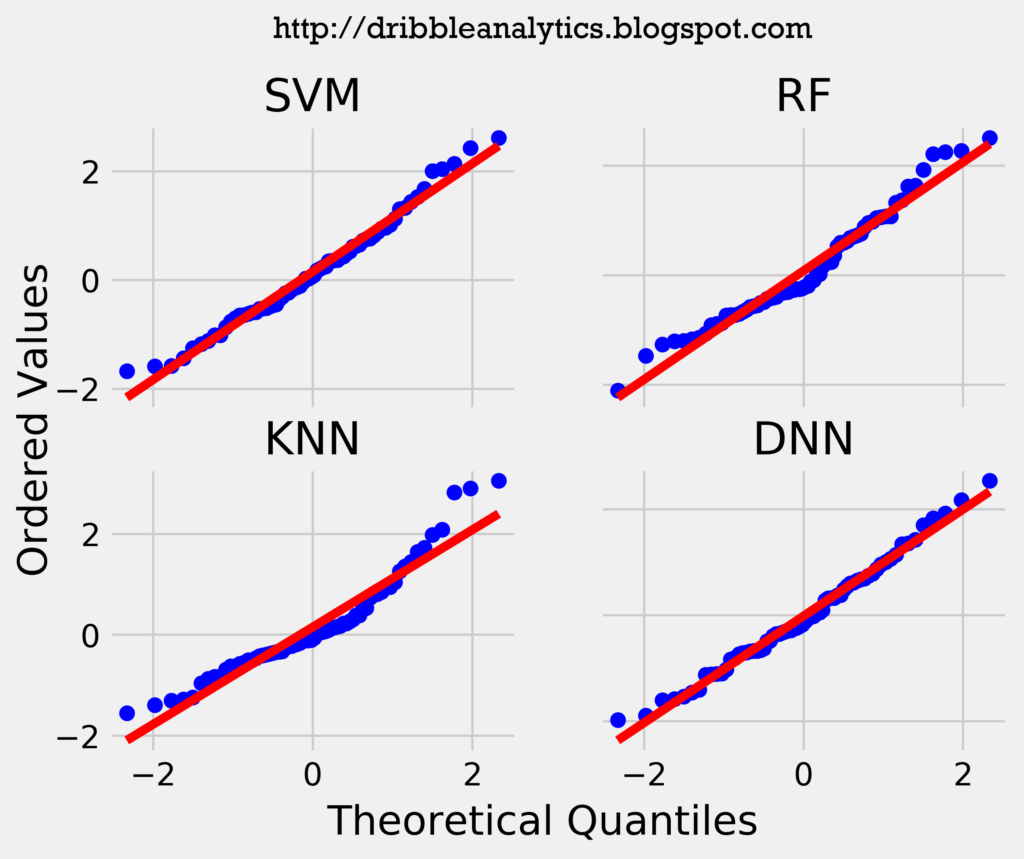
All four models’ Q-Q plot seems to have a nearly identical line to y = x. Furthermore, there are no noticeable jumps in the data. Therefore, from the Q-Q plot, it would appear that the residuals are normally distributed.
Shapiro-Wilk test
Though the Q-Q plots give us a general idea of whether our data is normally distributed, we can’t make a conclusion from just the plots. Therefore, I performed a Shapiro-Wilk test on the residuals. The test returns a W-value between 0 and 1. A W-value of 1 indicates the data is perfectly normal.
The test also returns a p-value for the null hypothesis that the data is normally distributed. Because the null hypothesis is that the data is normally distributed, a p-value < 0.05 indicates the data is not normally distributed (as p < 0.05 means we reject the null).
The table below shows the results of the Shapiro-Wilk test.
| Model | W-value | p-value |
|---|---|---|
| SVM | 0.98 | 0.37 |
| RF | 0.96 | 0.03 |
| KNN | 0.92 | 0.0004 |
| DNN | 0.99 | 0.67 |
Because p < 0.05 for the random forest and k-nearest neighbors, we can conclude that their residuals are not normally distributed. However, we can’t say the same for the support vector regression and deep neural network, as they have both very high W-values and high p-values. Therefore, it is likely their residuals are normally distributed.
Durbin-Watson test
One final consideration we will analyze is autocorrelation. The models’ residuals should have no autocorrelation; if the models do have significant autocorrelation, they are likely making the same mistake over and over again, and are therefore unusable. To test for autocorrelation, I performed a Durbin-Watson test. The test returns a value between 0 and 4. A value of 2 indicates no autocorrelation. Values between 0 and 2 indicate positive autocorrelation, and values between 2 and 4 indicate negative autocorrelation.
The table below shows the results of the Durbin-Watson test.
| Model | DW-value |
|---|---|
| SVM | 2.04 |
| RF | 2.13 |
| KNN | 2.04 |
| DNN | 2.15 |
All four models have a DW-value very close to 2. Therefore, it is unlikely that there is significant autocorrelation in the residuals.
Would we benefit from more data?
Theoretically, instead of training and testing the models with 1979-2007 data and then predicting with 2008-2018 data, I could train and test the models with all the years except the year we are trying to predict. In other words, to predict the 2018 MVP, I could either make models with my current set up, or introduce more data by making the models to include 1979-2017 data (instead of just 1979-2007).
To examine whether this model construction – which introduces more data – would increase the models’ accuracy, I plotted the learning curves for mean squared error (MSE) and r-squared for the models.
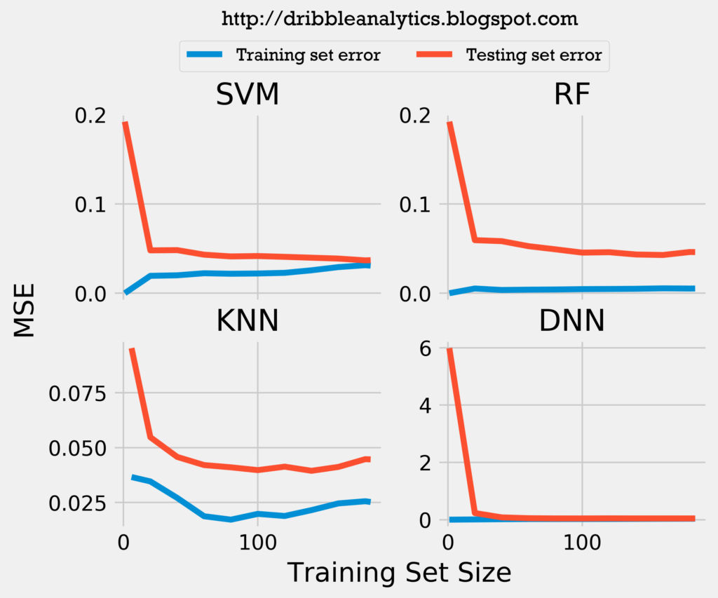
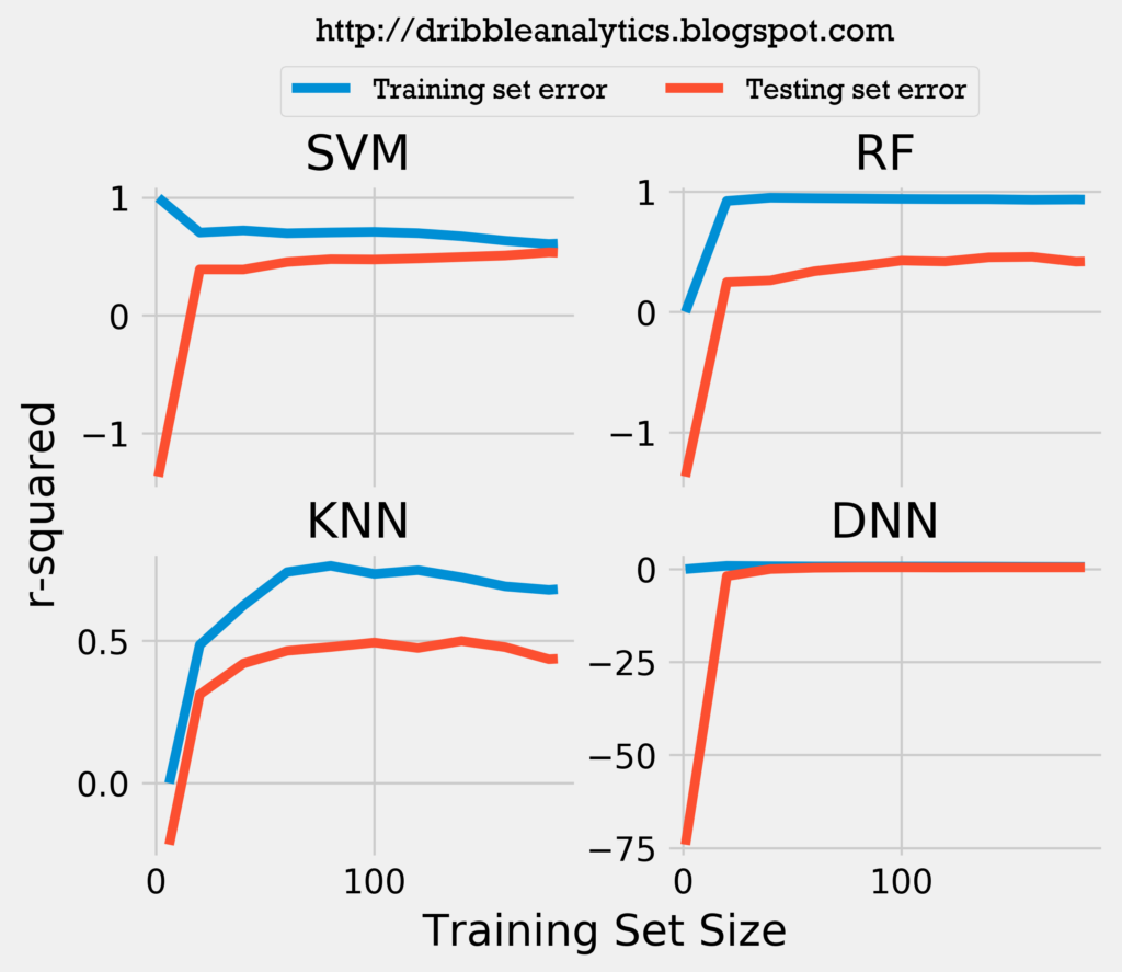
Because the training and testing set error lines converge to a near identical position for the SVM and DNN, it is unlikely that adding more data would increase the accuracy of the support vector regression and the deep neural network. However, it could increase the accuracy for the random forest regression and k-nearest neighbors regression. Therefore, constructing the model differently to introduce more data does not drastically increase the accuracy.
Results
The results for each year will be displayed by graphs of each model’s predictions, followed by the average of these predictions.
2007-2008
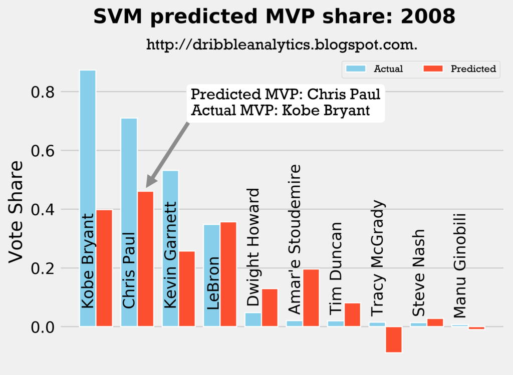
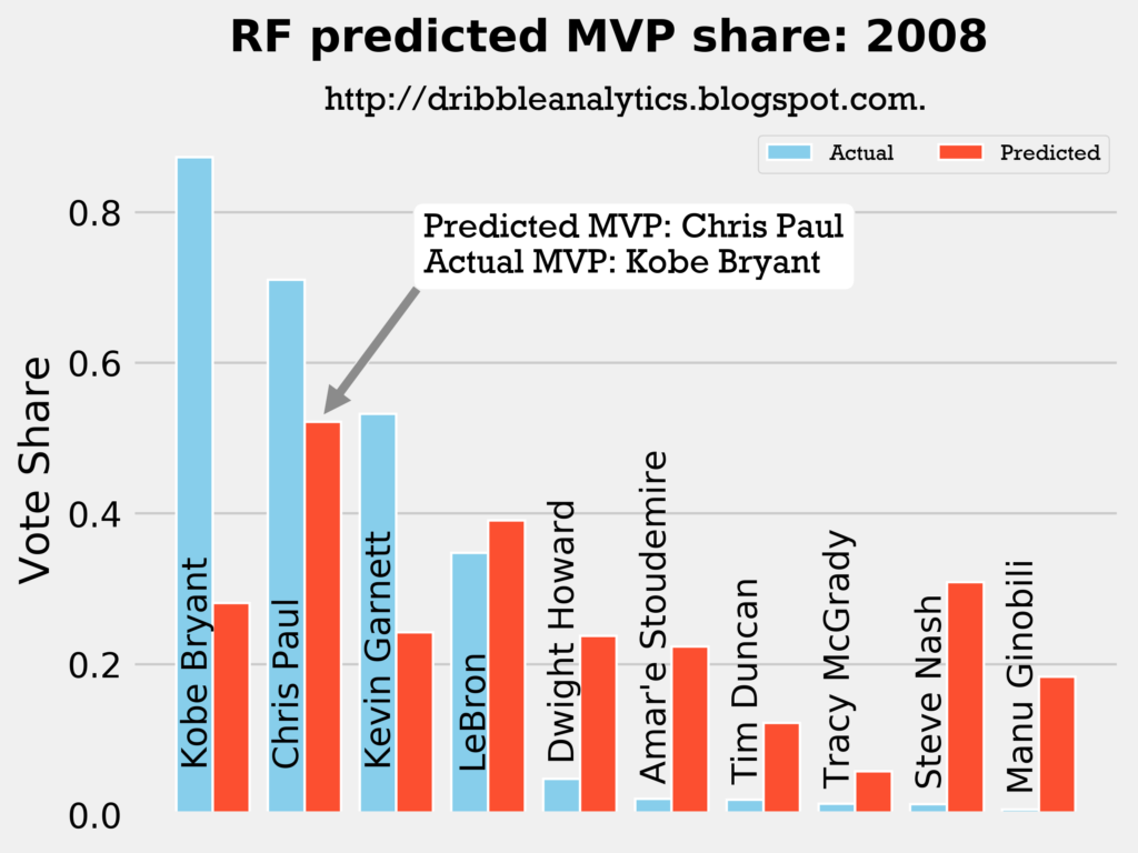
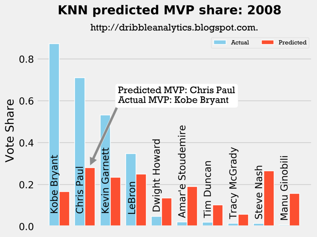
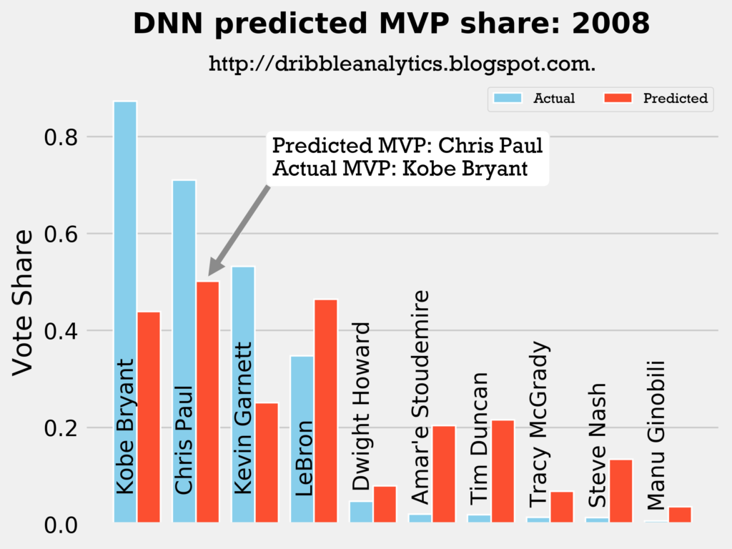
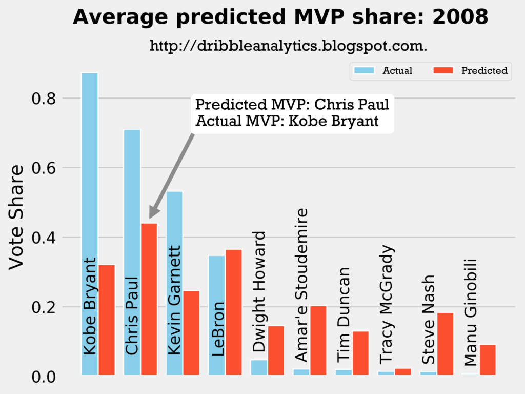
Result: all four models say Chris Paul should have won MVP over Kobe.
2008-2009
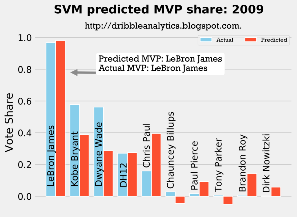
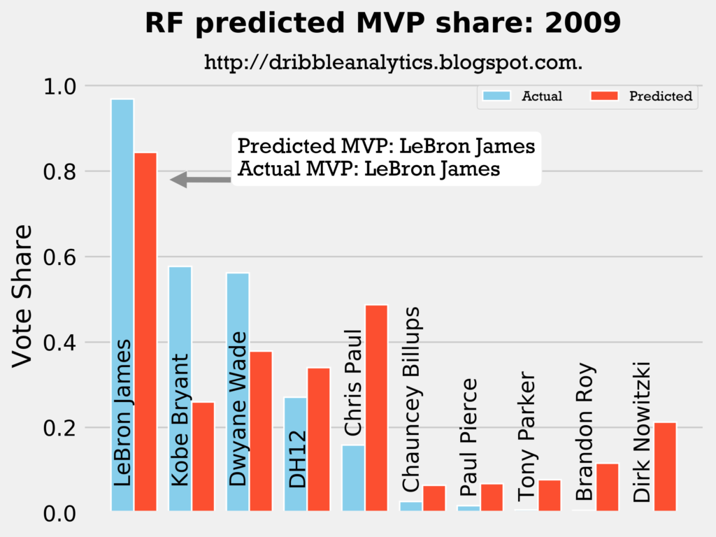
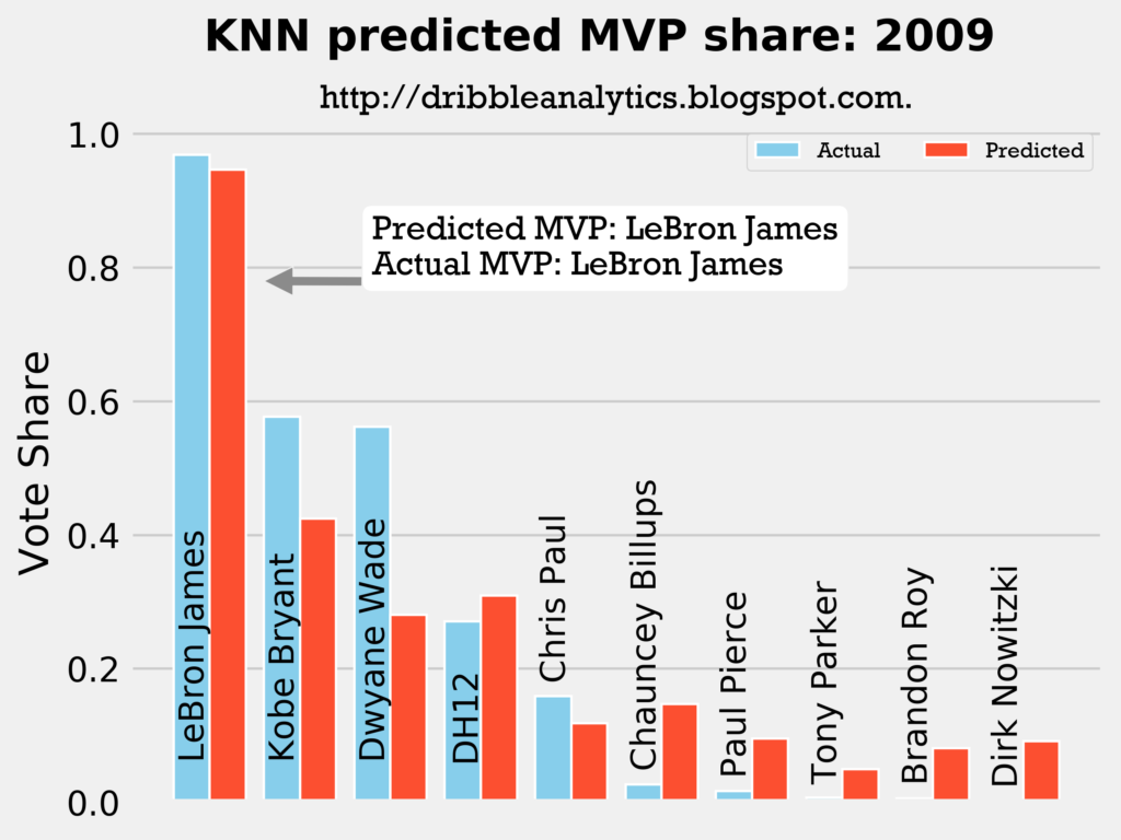
Result: all four models say LeBron still wins MVP.
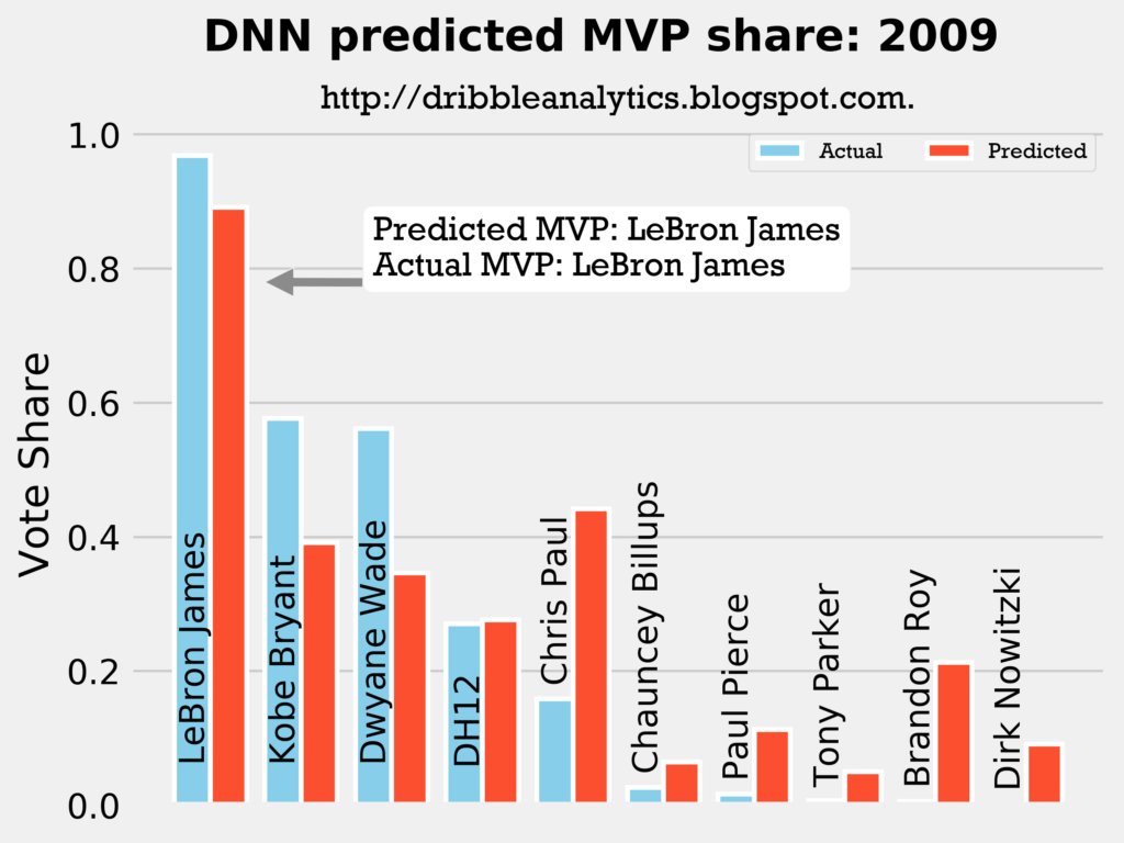
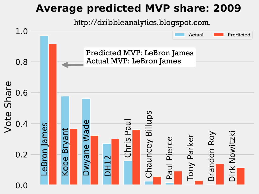
2009-2010
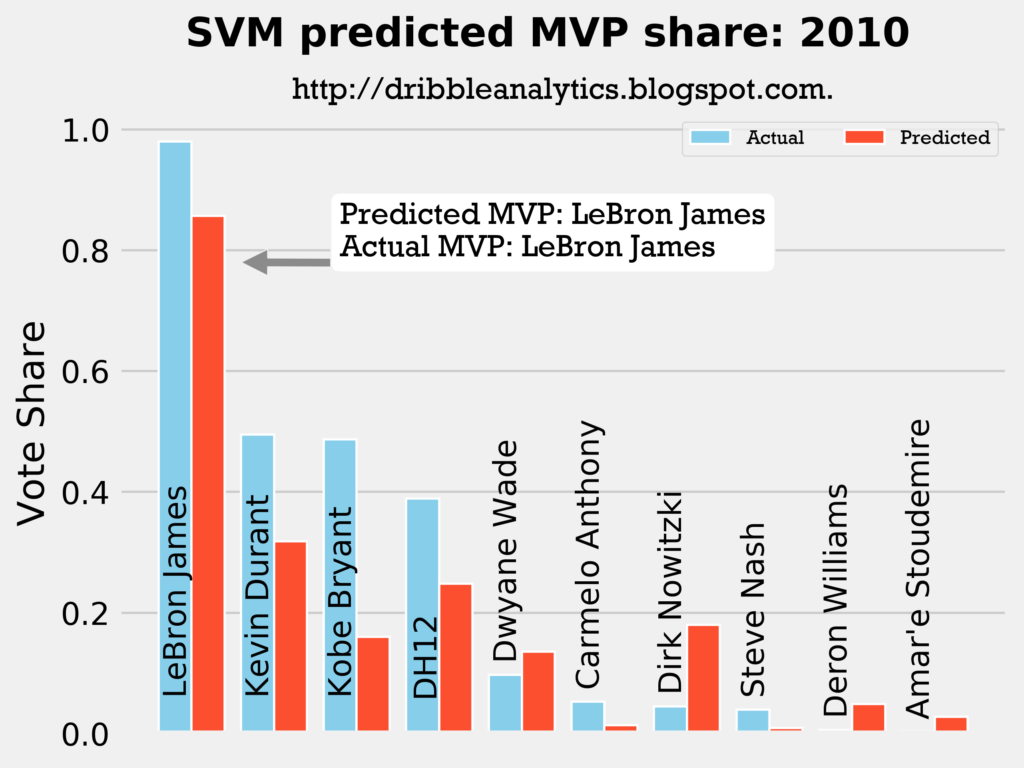
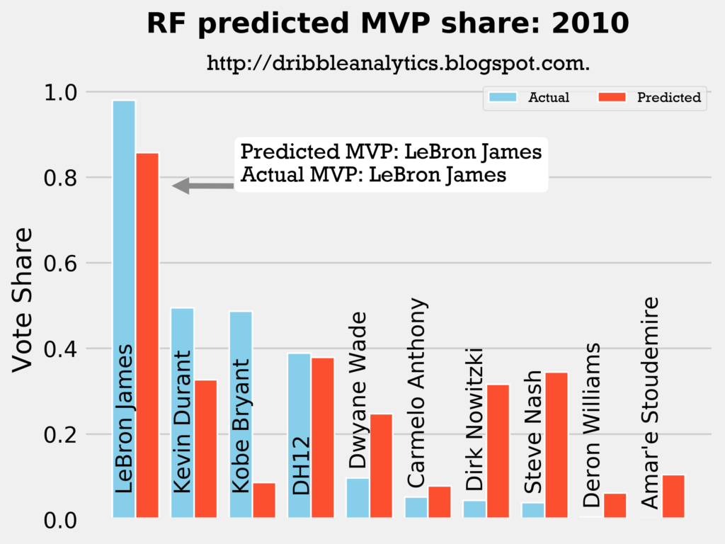
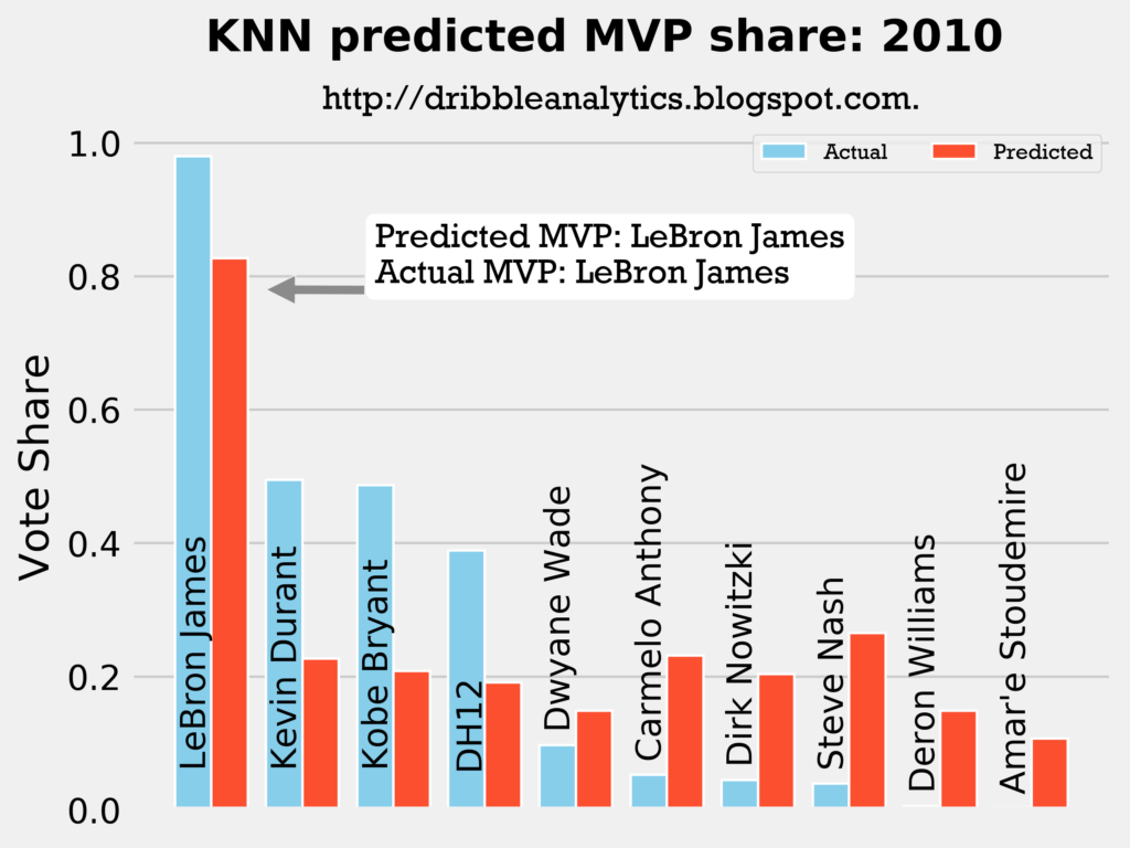
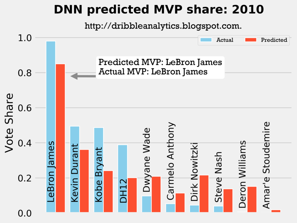
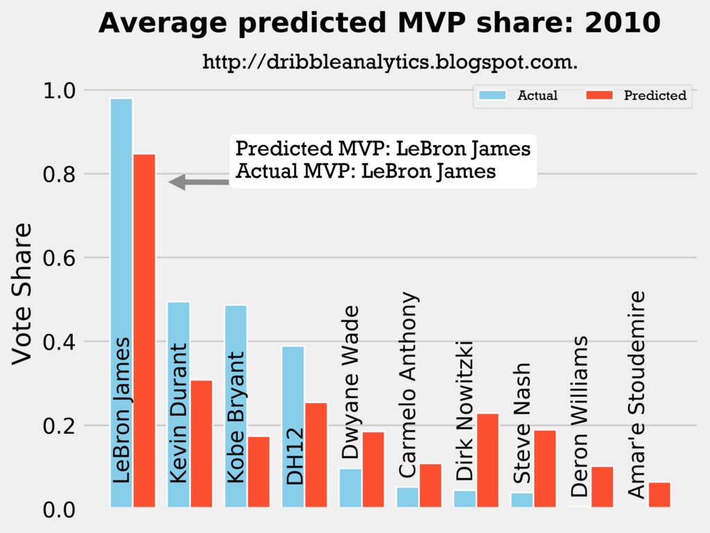
Result: all four models say LeBron still wins MVP.
2010-2011
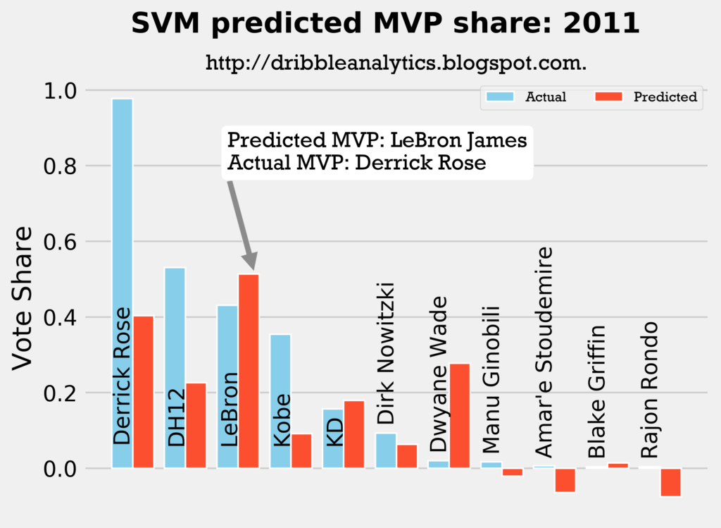
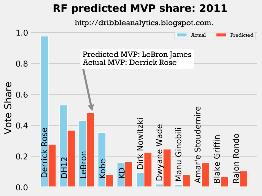
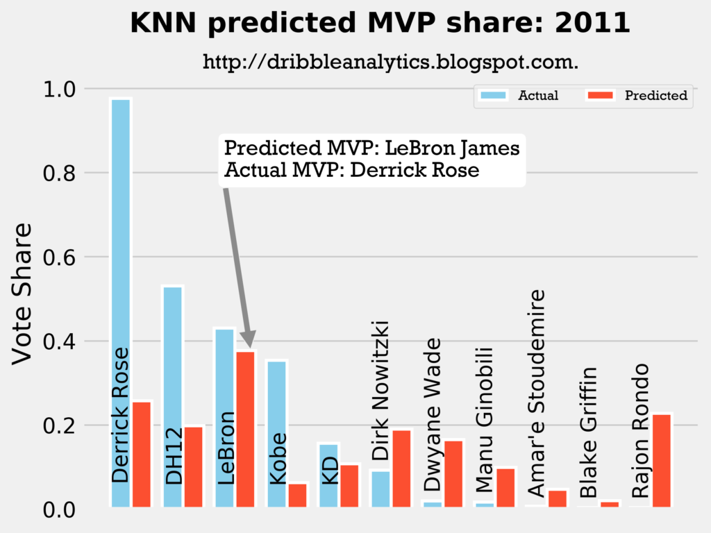
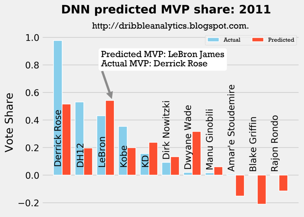
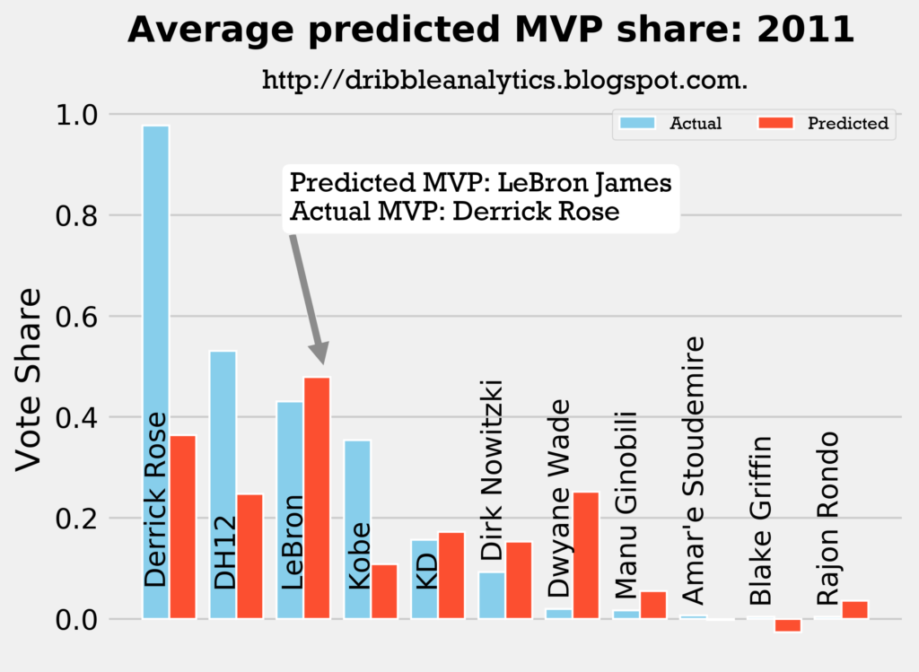
Result: all four models say LeBron should have won MVP over Derrick Rose.
2011-2012
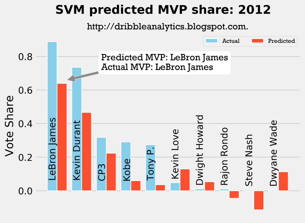
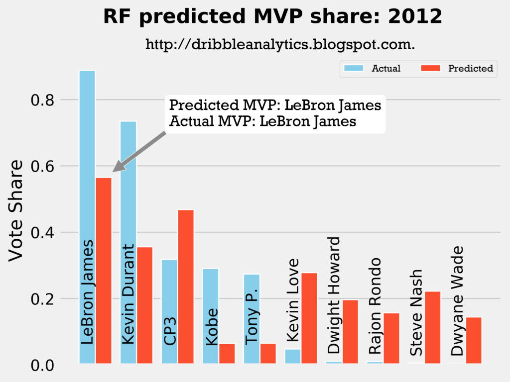
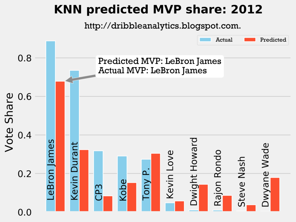
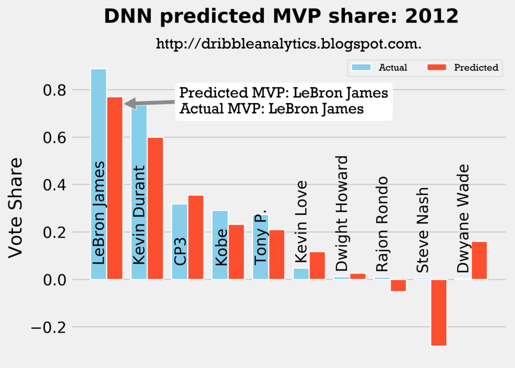
Result: all four models say LeBron still wins MVP.
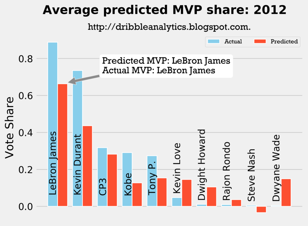
2012-2013
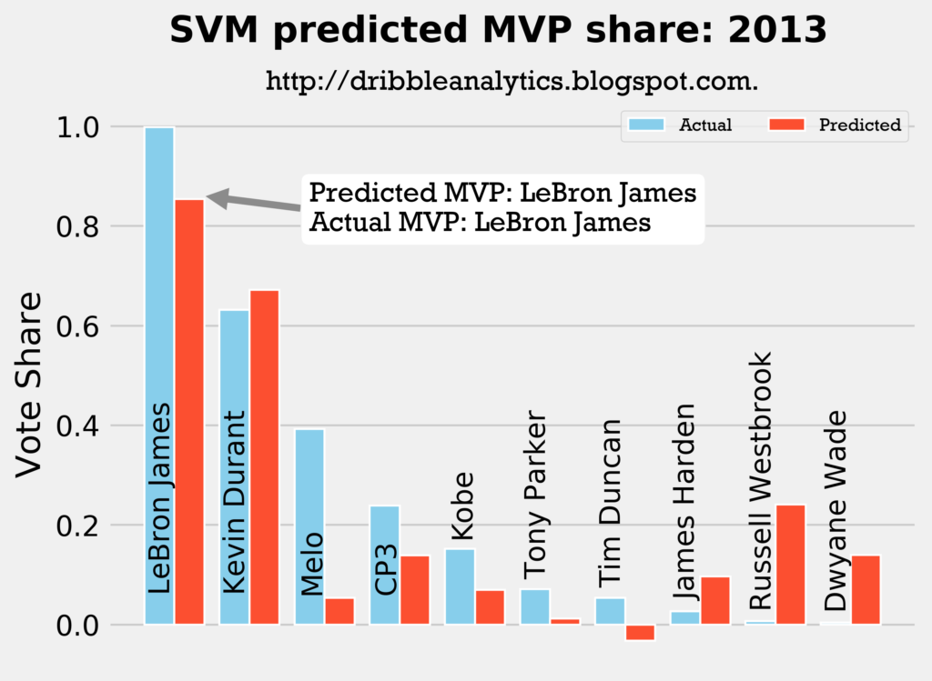
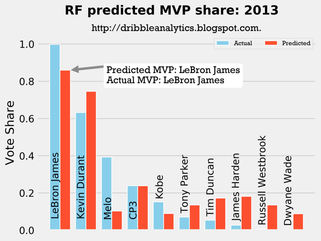
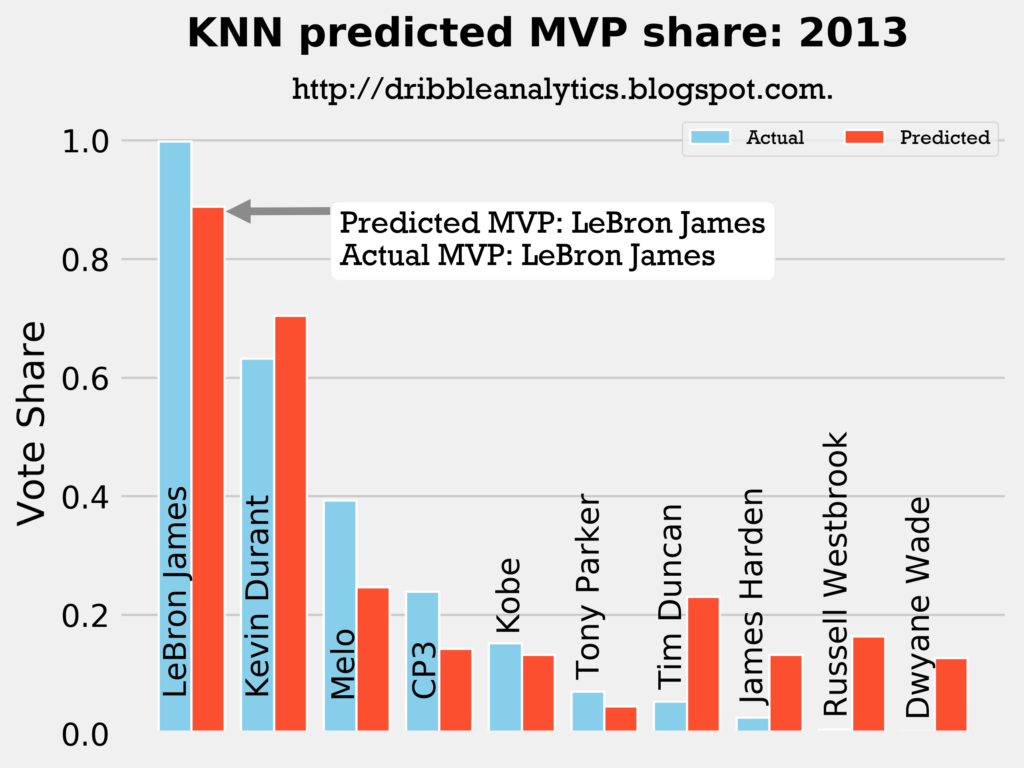
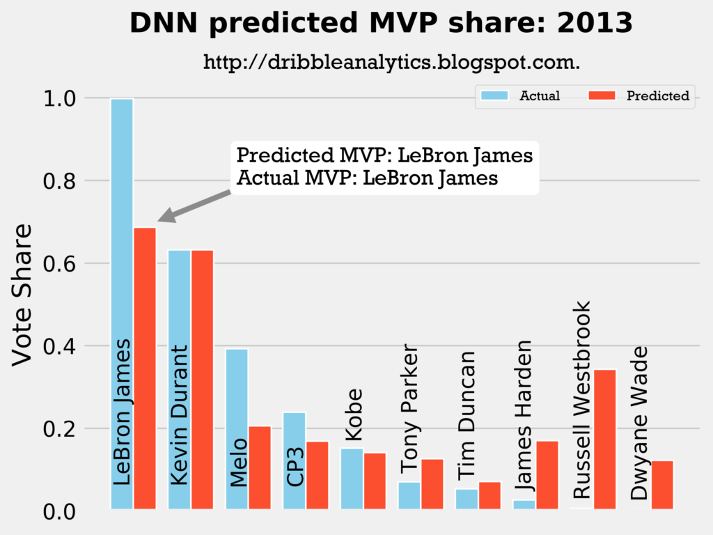
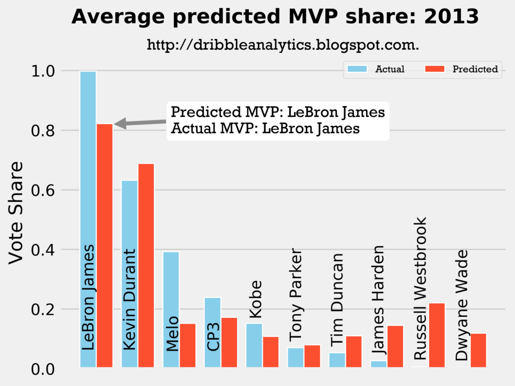
Result: all four models say LeBron still wins MVP.
2013-2014
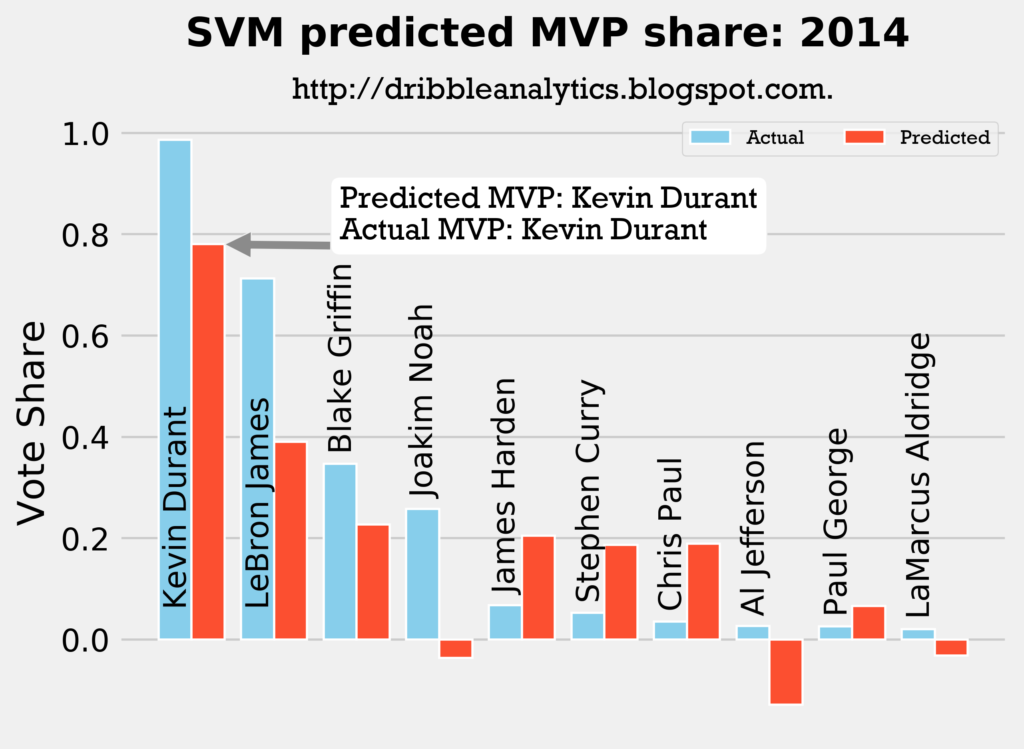
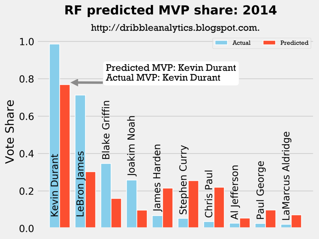
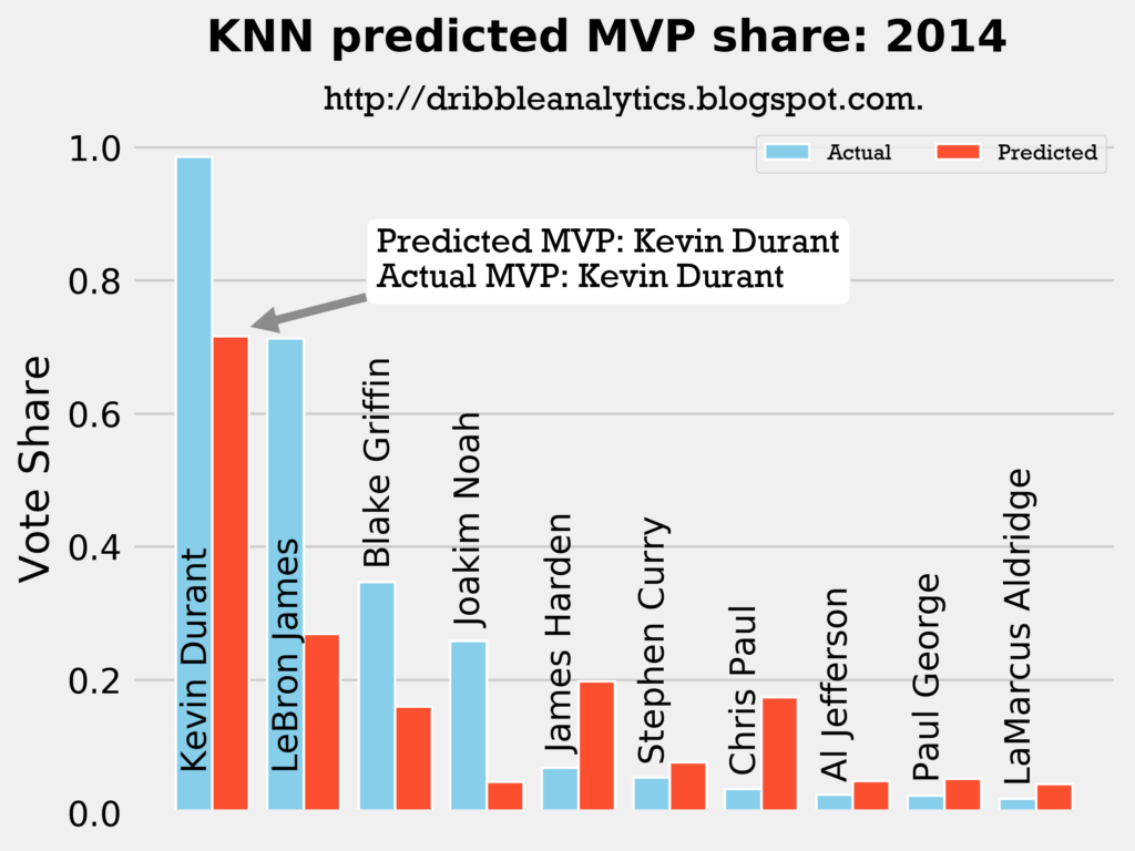
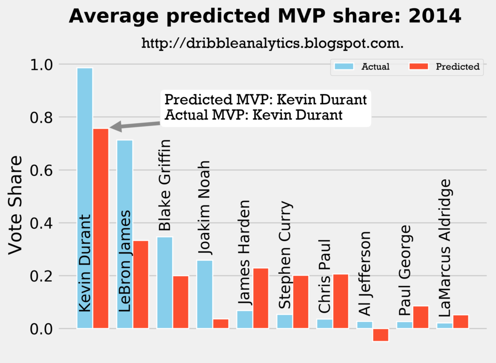
Result: all four models say Kevin Durant still wins MVP.
2014-2015
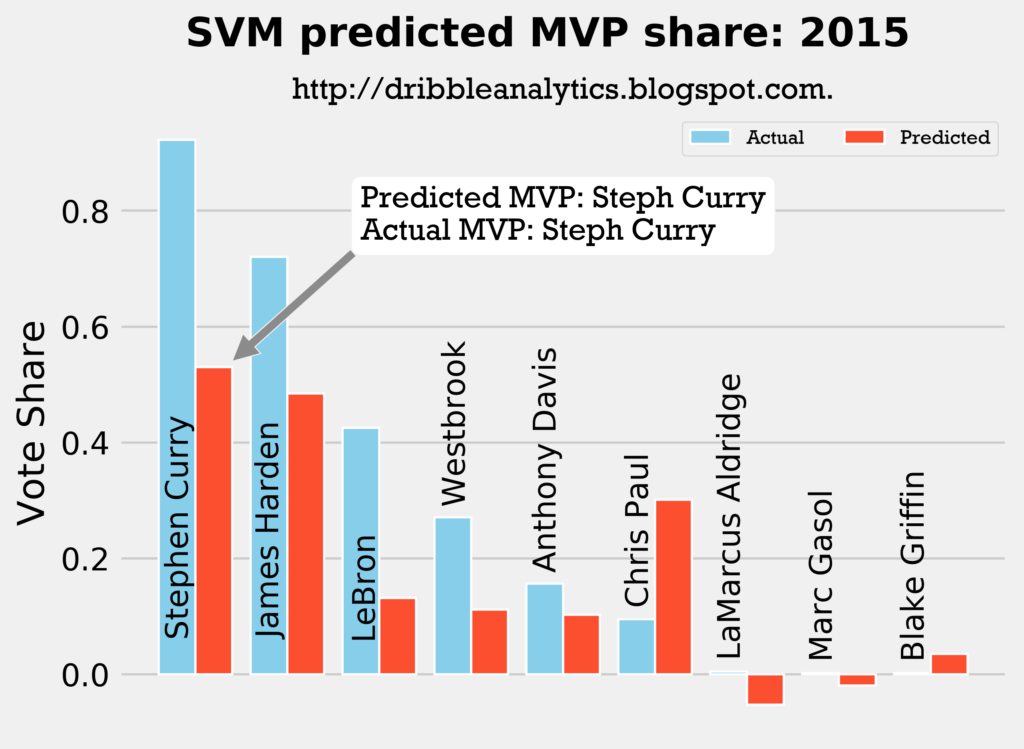
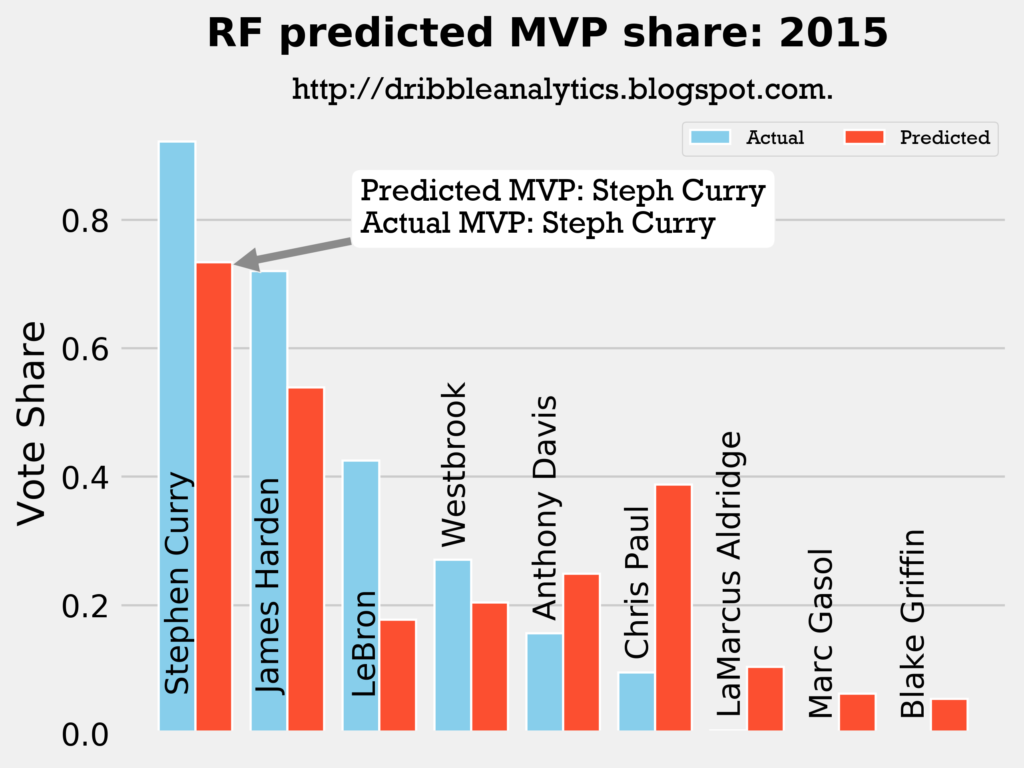
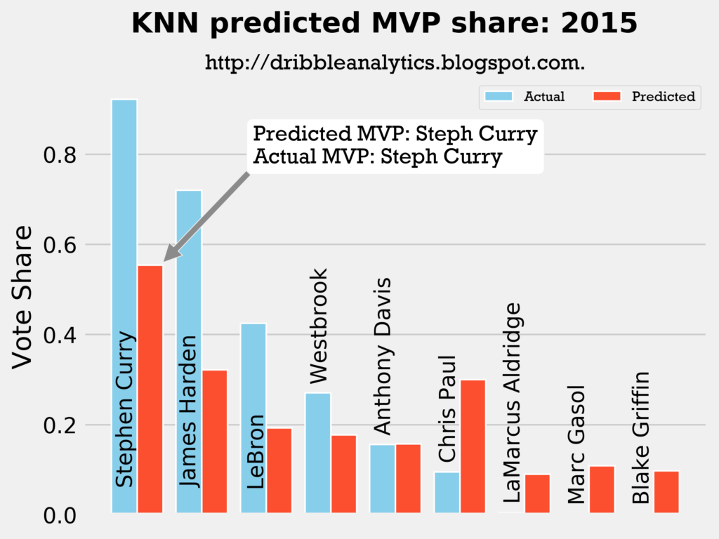
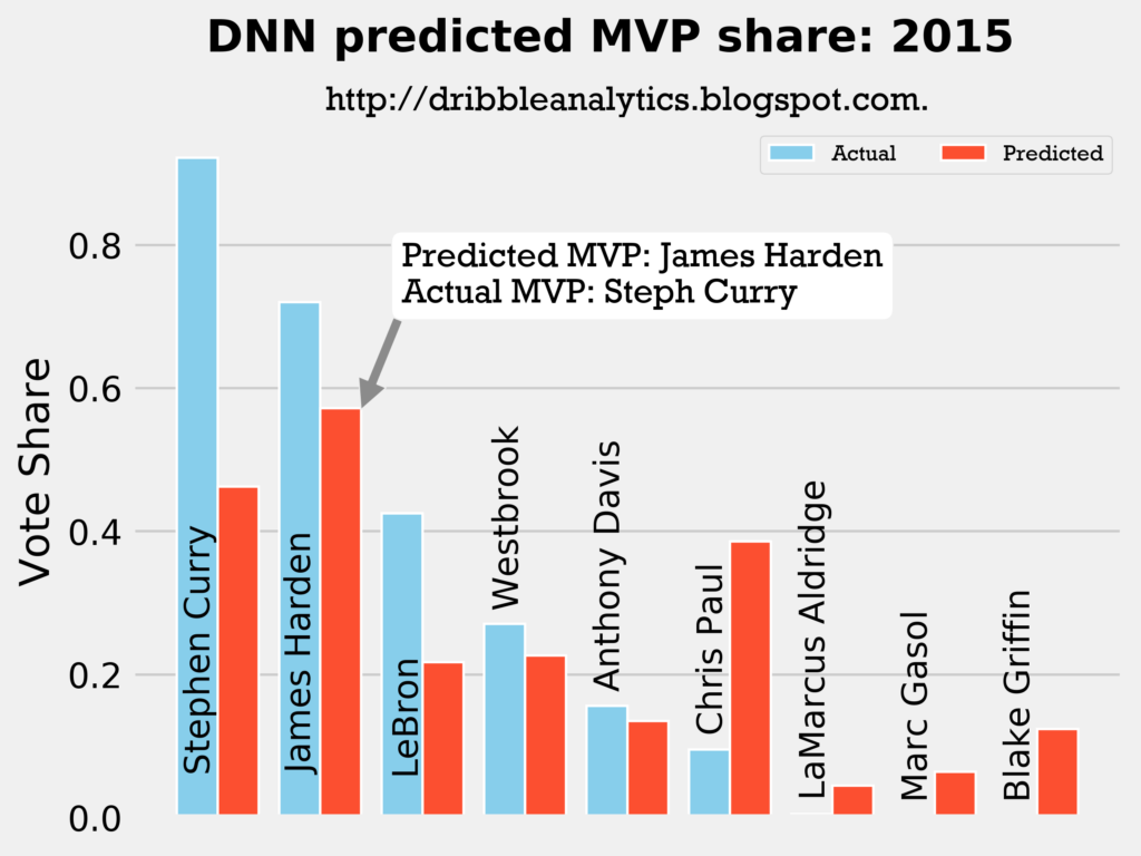
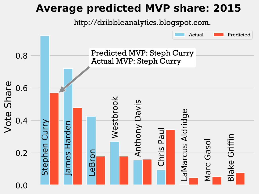
Result: the DNN thinks Harden should have won MVP, but the other three models (and the four-model average) say Curry still wins MVP.
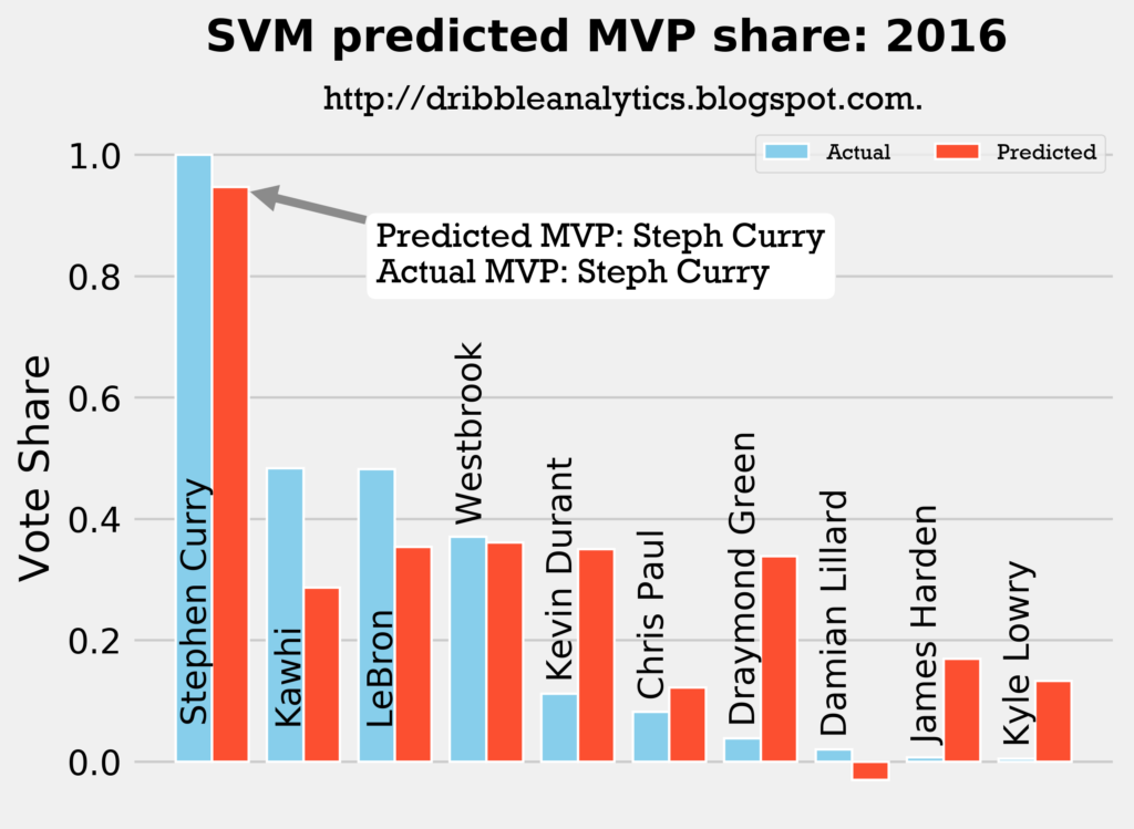
2015-2016
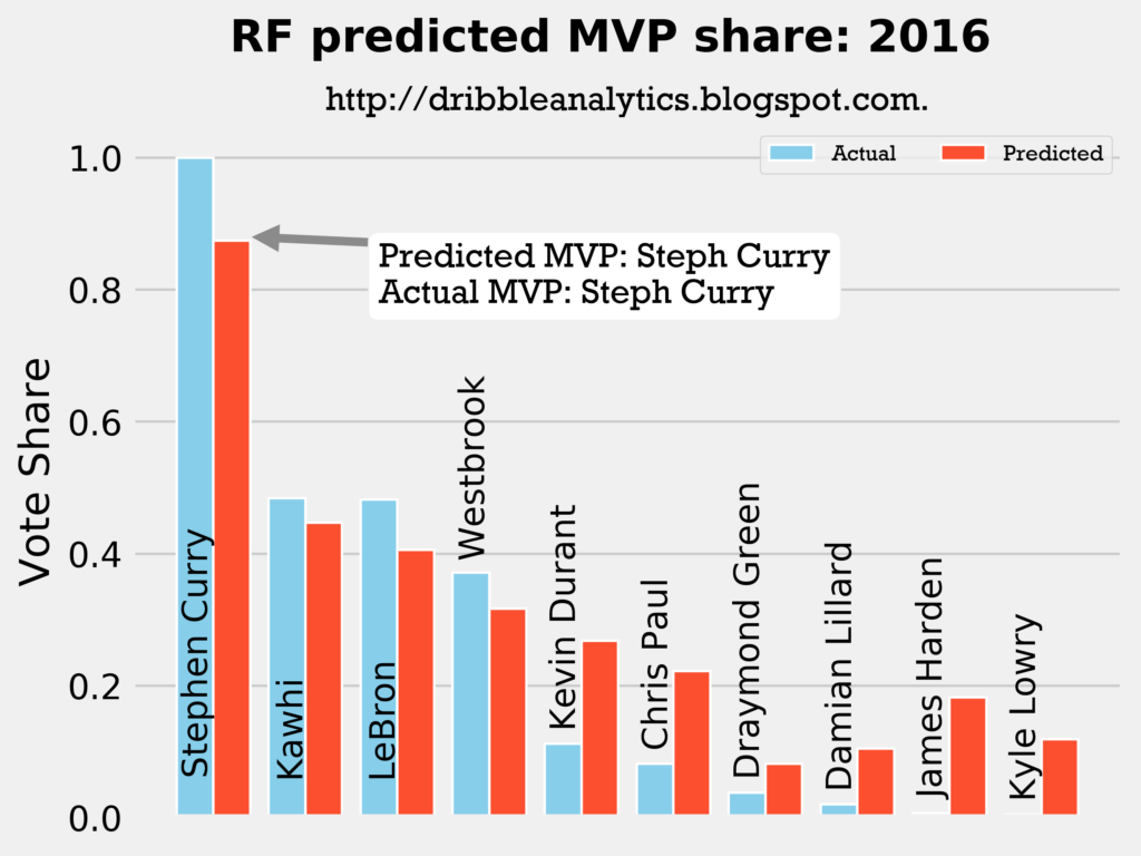
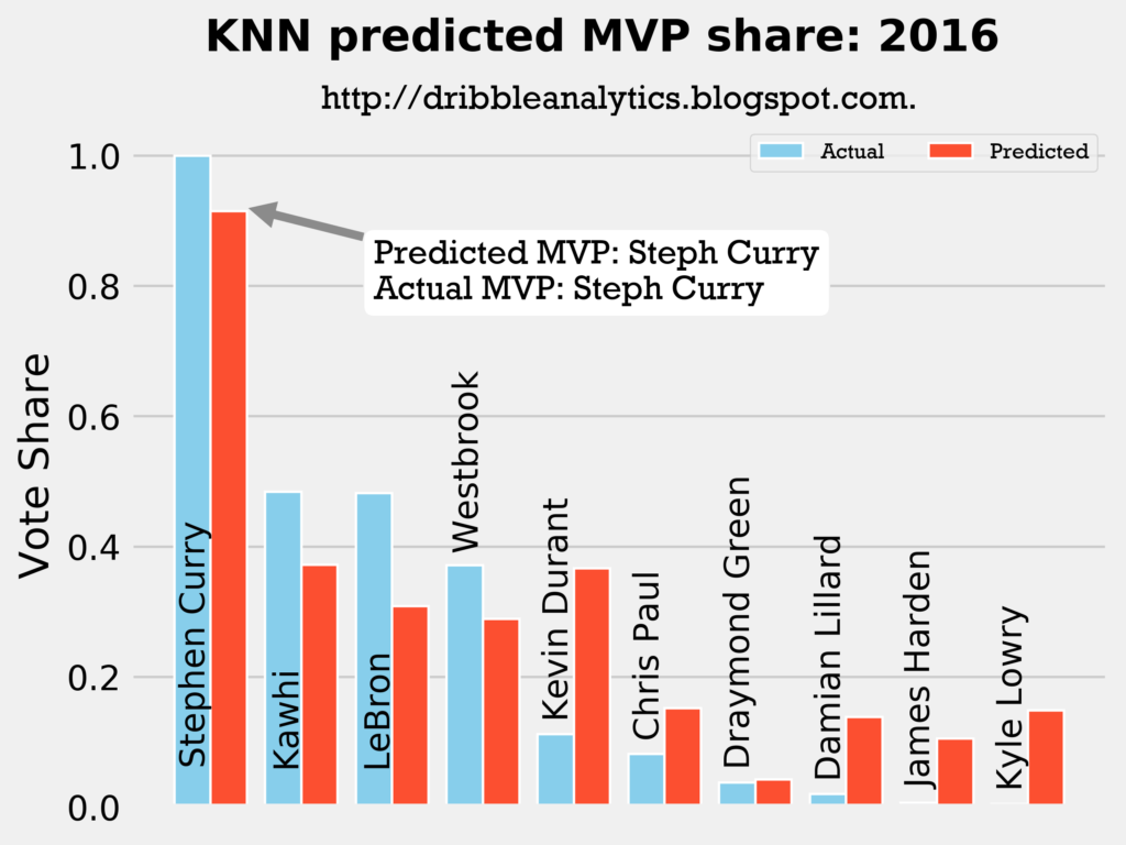
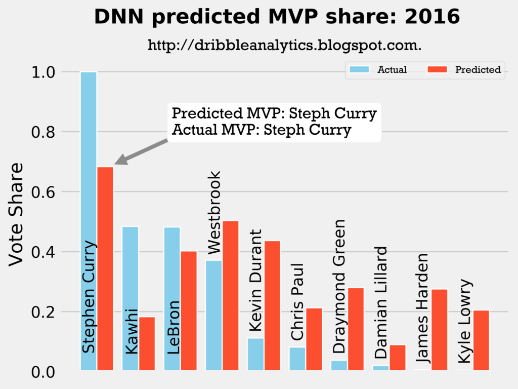
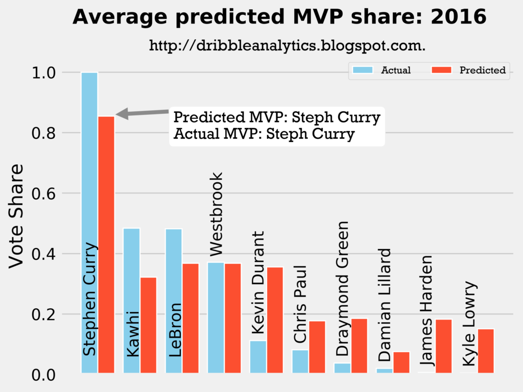
Result: all four models say Curry still wins MVP.
2016-2017
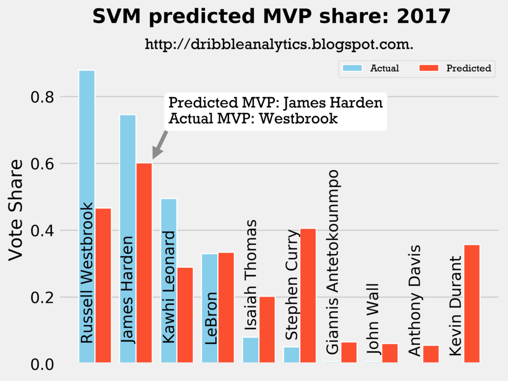
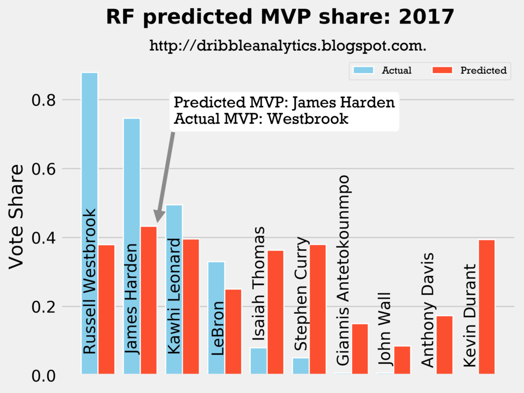
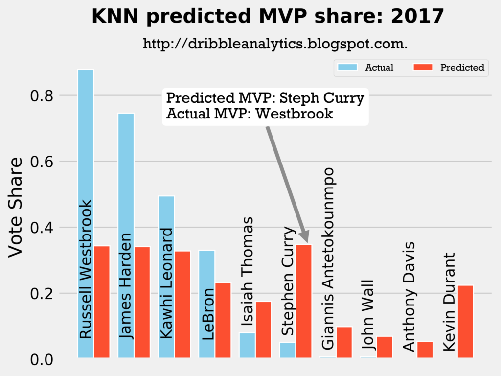
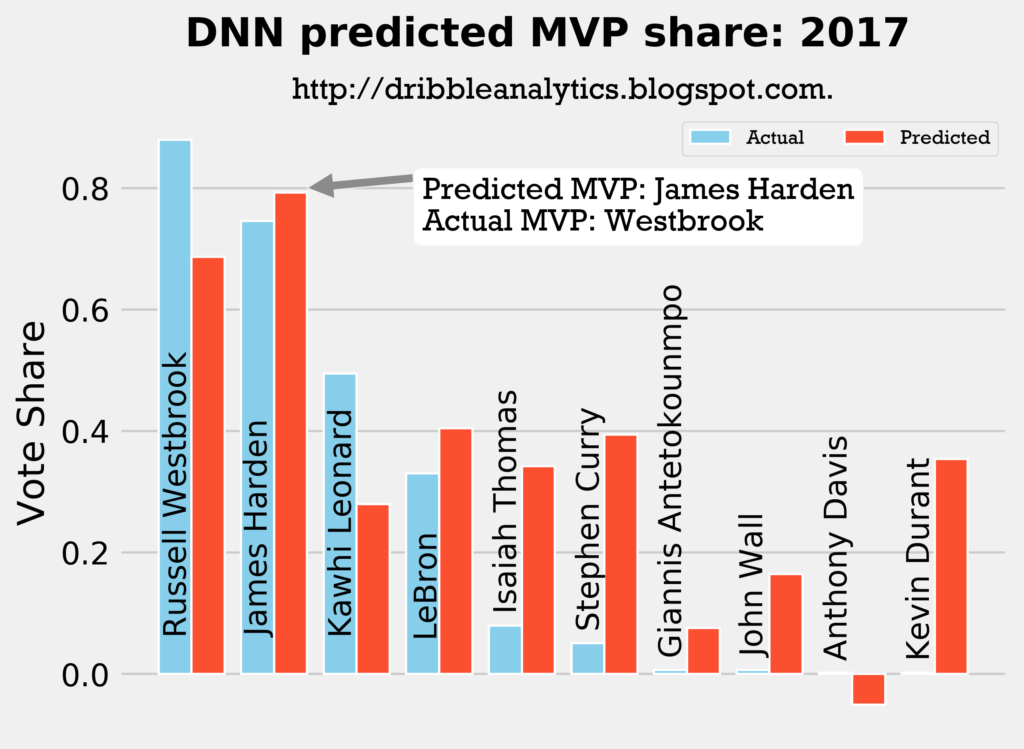
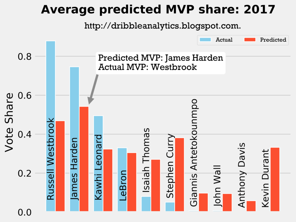
Result: the k-nearest neighbors regression says Curry should have won over both Harden and Westbrook. The other three regressions (and the four-model average) say Harden should have won MVP over Westbrook.
2017-2018
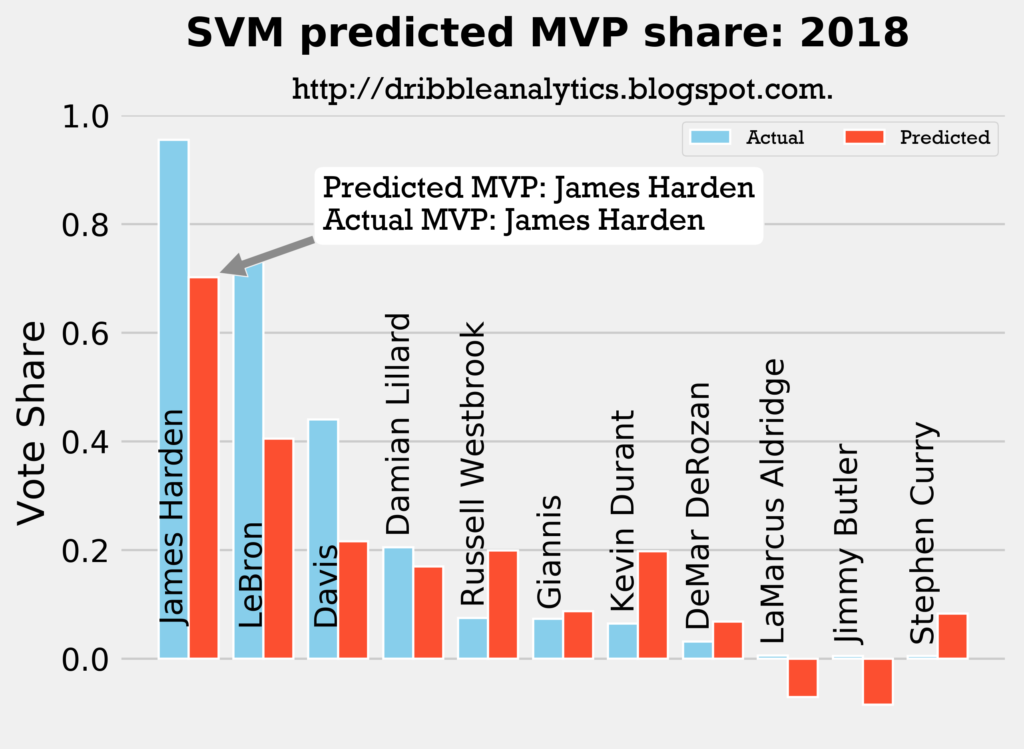
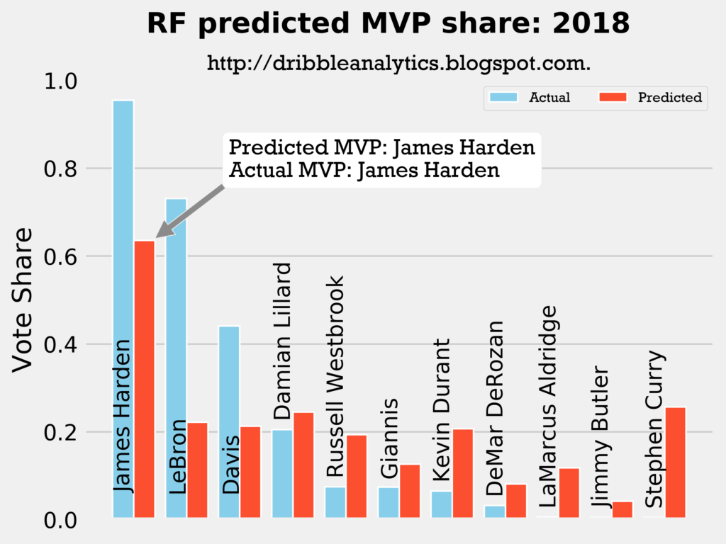
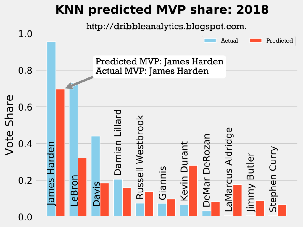
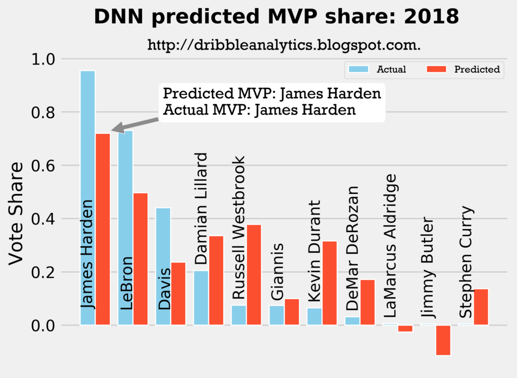
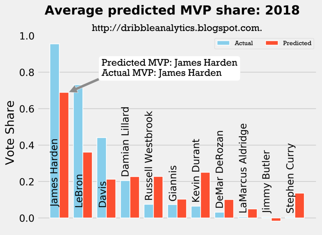
Result: all four models say Harden still wins MVP.