Summary


Introduction
Previously, we used machine learning to predict the best shooters and defenders in the 2018 draft. While predicting the best distributors is similarly challenging to predicting the best shooters and defenders given the different types of offenses in college, there is an additional challenge in predicting distributors. Distribution skills are largely intangible.
Defense is also largely dependent on intangibles (hustle and effort), but we can measure what makes a good defender (advanced stats for defense are very poor, but we still know that generally a player who gets a lot of steals is better than one who gets none).
Distribution is very dependent on passing vision. Because we don’t have objective stats to measure vision, it’s very difficult to predict a player’s distribution skills. Furthermore, a player’s ability as a floor general depends on their leadership – also immeasurable with stats. Lastly, not all assists are created equal. For example, some players clearly pad their assist stats. Also, an assist doesn’t measure a player’s ability as a passer; a simple pass swinging it across the perimeter when the defense misses a rotation is worth the same as a difficult pass through traffic.
Given these factors, it is difficult to measure a player’s ability as a distributor, and even harder to predict how well a college player’s assists and turnovers will translate to the NBA.
Similar to how a zone may inflate a center’s defensive stats in college, different offensive schemes create variance in a college player’s distribution stats. For example, a point guard might have very high assist numbers because his offense runs a pick-and-roll heavy scheme featuring a dominant big man. So, while his stats show he is a good distributor, in reality the stats are inflated because of his team.
Despite all these issues, assists and turnovers remain our best ways to measure a player’s distribution skills. Though in the NBA, stats such as offensive rating can be used, college teams play at vastly different paces, thereby making offensive rating a potentially poor representation of a player’s offensive effect. Therefore, assists and turnovers are the best numerical representation of whether a player is a good distributor. Using several distribution statistics and other factors, we can try to predict the 2018 draft’s assists and turnovers, giving us a good idea of who the best distributors in the draft are.
Methods
First, I used a Basketball Reference draft finder to pull up all guards drafted in the first round who played in college since the 2003 draft. The 2003 draft is set as the limit because players drafted before then have no college data for AST%. For the 133 players who showed up in the search, I recorded the following stats:
| College stats | NBA stats | Other information |
|---|---|---|
| MPG | MPG | Pick selected |
| AST | AST | Age at draft |
| TOV | TOV | Height (in) |
| AST/TOV | AST/TOV | |
| AST% | AST% | |
| TOV% | TOV% | |
| SOS |
For the 2018 draft class, I recorded the college stats and other information for all players who ESPN listed as guards on their draft summary.
Though shooting guards sometimes don’t have facilitating roles in an offense, I included them given that it is still important that they limit turnovers, and slashing shooting guards should be able to have the defense collapse on them (thereby creating assists).
With the dataset complete, I created 4 different machine learning models to predict assists and turnovers:
- Linear regression
- Support vector regression
- Random forest regression
- k-Nearest neighbors regression
The model used all the college stats and other information as inputs except for MPG and AST/TOV. Assist to turnover ratio was excluded because it is a result of two other inputs in the model (assists and turnovers), thereby creating an issue with multicollinearity.
Using these inputs and model types, I created models to predict assists and turnovers. 80% of the dataset was used to train the models, and the remaining 20% was used to test the models’ accuracy.
Comparing college and NBA stats
Though assists largely depends on intangibles and offense, the correlation between assists in college and the NBA is not very poor. This may be because players aren’t likely to “lose” the intangibles. However, the correlation is not very strong. The graph below shows the correlation between college and NBA AST/G for all the 133 players in the dataset.
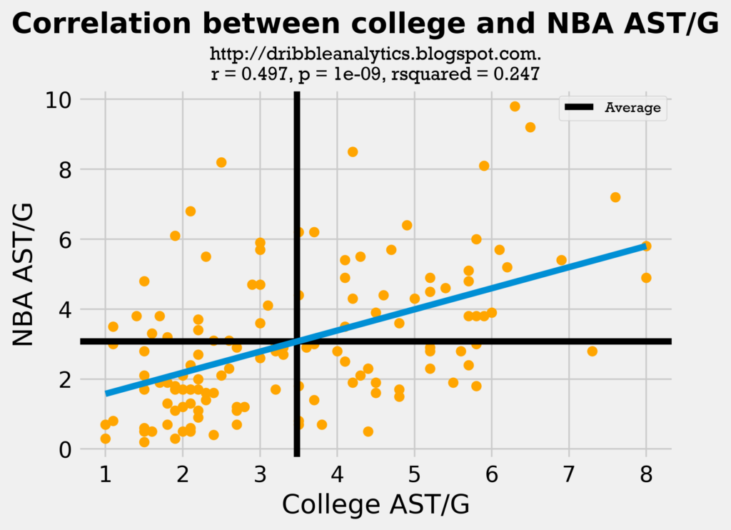
The regression is statistically significant (p-value < 0.05). However, the correlation coefficient (r) is very weak, and the low rsquared indicates a weak model.
The graph below shows the correlation between college and NBA TOV/G.
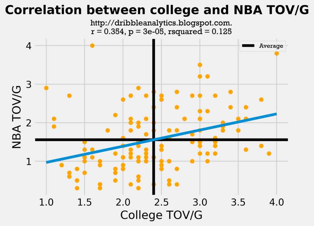
This regression is even weaker than the assists regression. The graph below shows the correlation between college and NBA AST/TOV.
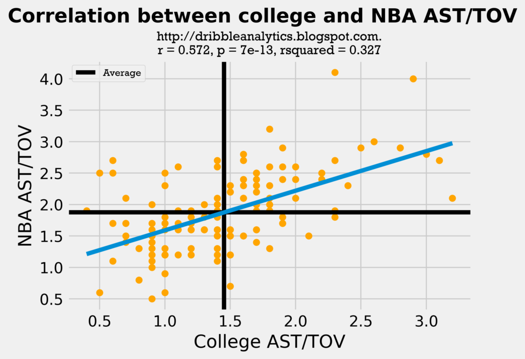
Though this regression is the strongest of the three, it is still very weak. The correlation coefficient is still low.
While all regressions are statistically significant, they are not very accurate. It is important, however, to establish that the comparison between the sample’s college stats and the draft class’s stats is fair.
To examine the fairness of this comparison, let’s look at histograms of assists and turnovers for our current players dataset in both college and the NBA, and for our draft class dataset. If the distributions look similar, and the mean and standard deviation are close between our sample’s histograms and the draft class’s histogram, then we can suspect the comparison is fair.
First, let’s look at histograms for assists.
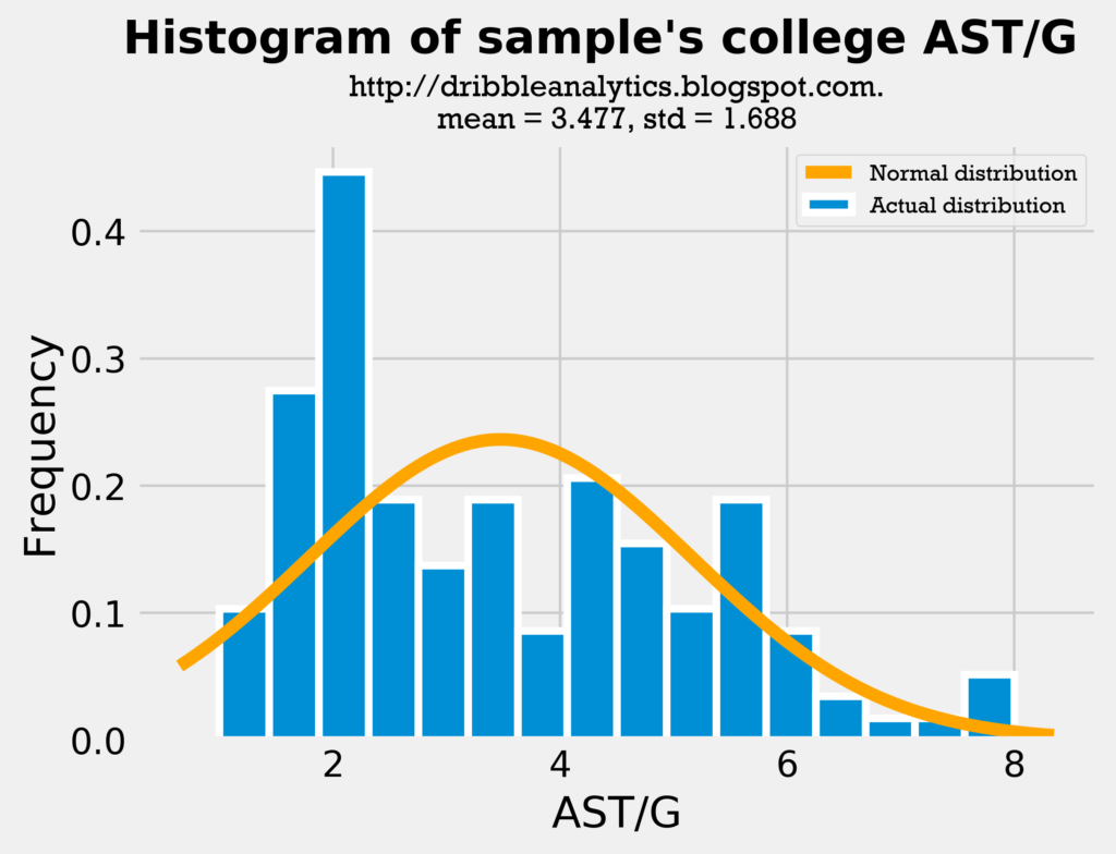
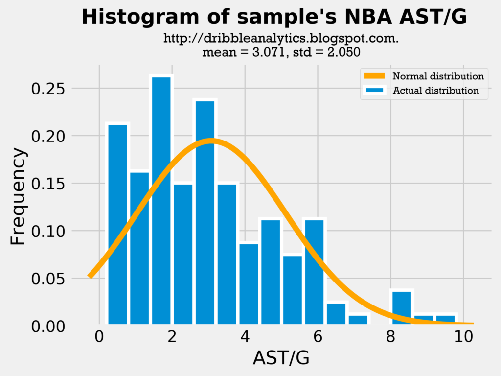

The mean and standard deviation in our sample’s college AST/G and the draft class’s AST/G is very close. Furthermore, the distributions look similar; most players have around 2-4 assists, and then about one player a year has around 8 assists.
The graphs below are the histograms for turnovers.
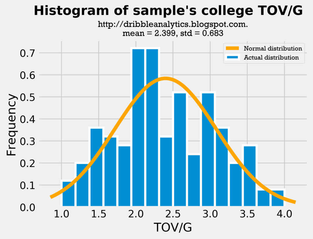
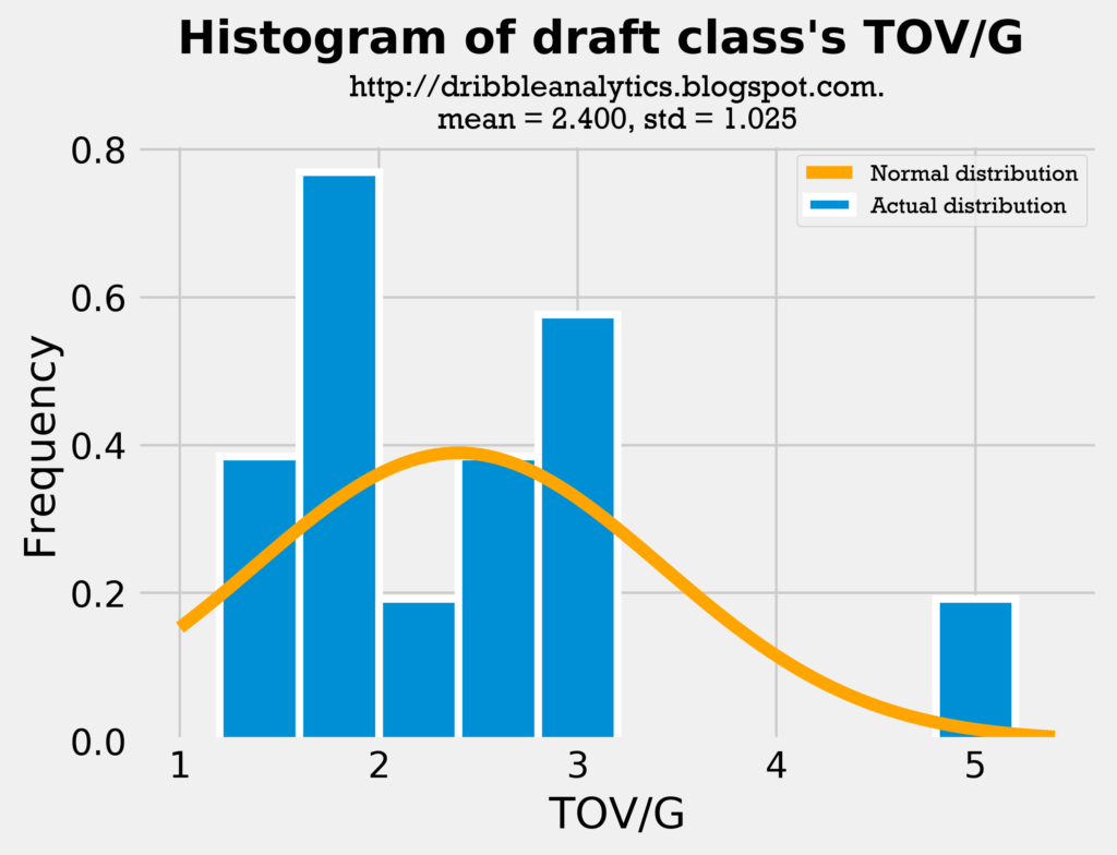
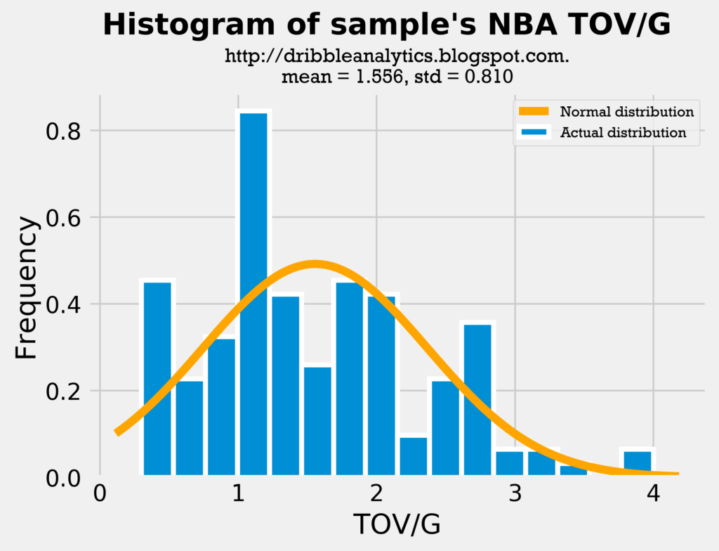
The mean for the sample’s college TOV/G is almost identical to the mean for the draft class’s TOV/G. Though the distribution looks slightly different and the draft class has a higher standard deviation, this is largely due to Trae Young’s high turnover count.
Therefore, both the assists and turnovers histograms show the comparison between the sample and the draft class is fair.
Model accuracy: assists
Rsquared, mean squared error, and cross-validation
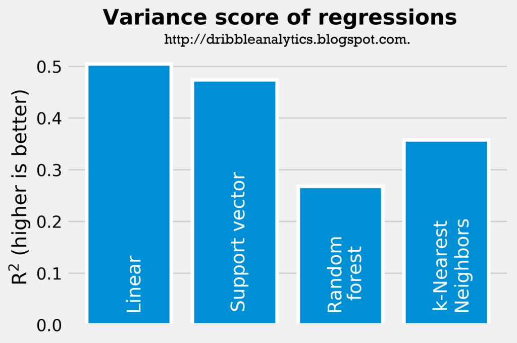
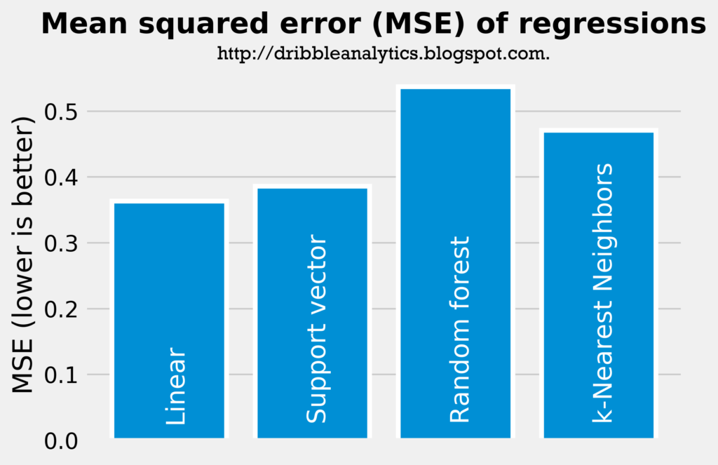
The two graphs below show the rsquared and mean squared error of the four regressions. Note that a higher rsquared indicates a smaller error in the models, while a lower mean squared error indicates a smaller error.
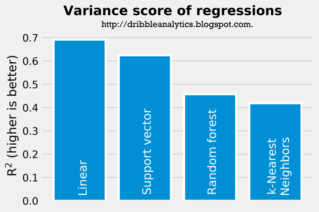
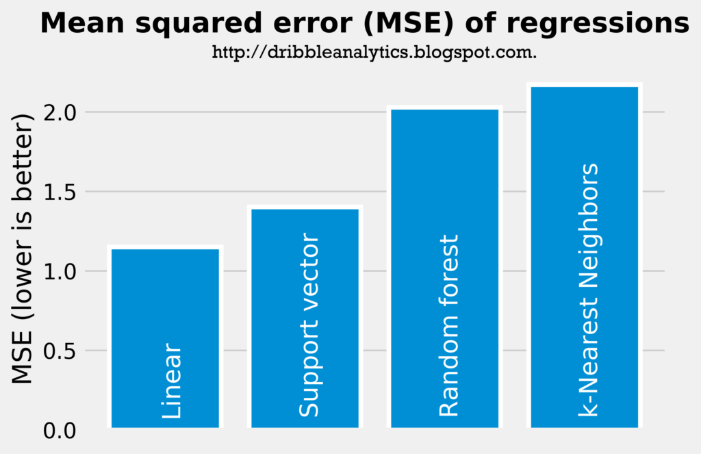
The rsquared and mean squared error indicates that the linear regression has the smallest error, followed by the support vector regression, random forest regression, and k-Nearest Neighbors regression, respectively. Though none of the rsquareds are particularly high, they are all much higher than the rsquared from the simple correlation between college and NBA assists.
To test for overfitting (i.e. testing that the models didn’t just learn to have the highest accuracy for our specific test set), I used k-Fold cross-validation (with n_splits = 4). I examined the models’ cross-validation scores for explained variance to see which models (if any) are overfitting.
The linear regression had a cross-validation score of 0.43, with the 95% confidence interval being +/- 0.50. The support vector regression had a cross-validation score of 0.61, with its 95% confidence interval at +/- 0.09. The cross-validation scores for the random forest and k-Nearest Neighbors regressions were 0.43 and 0.50, respectively. The 95% confidence intervals were +/- 0.62 and +/- 0.28 respectively.
All four models had their rsquared inside the 95% confidence interval for explained variance. While the linear regression’s cross-validation score was significantly lower than its rsquared (0.43 vs 0.692), the other models had their cross-validation scores either lower by a small margin (< 0.02 for the support vector and random forest regressions) or higher (for the k-Nearest Neighbors regression).
Therefore, the linear regression might be overfitting to some extent, while the other models are not.
Residuals tests
An important consideration in the models’ accuracy is that the models must have random and normally distributed errors. If the errors are not random or normally distributed, then the models are skewed in some way, and are therefore less accurate.
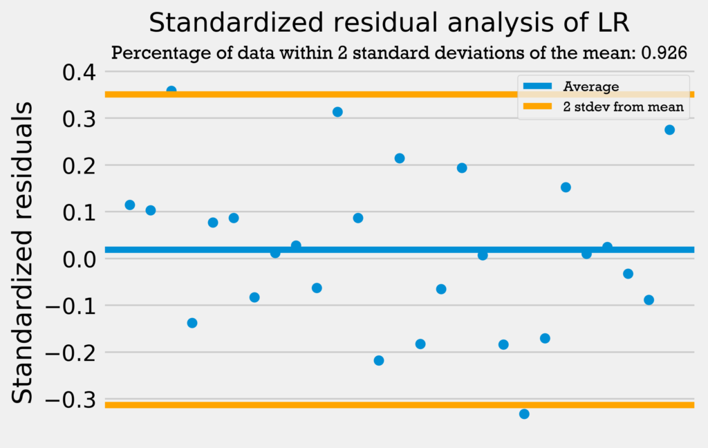
The first residuals test I performed was a standardized residuals test. In a standardized residuals test, the residuals from a regression model are standardized and measured. A very high standardized residual (> 2) or low (< -2) indicates an issue with the observed frequency.
So, we’re looking for the standardized residuals to be mostly between -2 and 2. Also, a general rule of thumb is that 95% of the data should be within 2 standard deviations from the mean if the data is normally distributed.
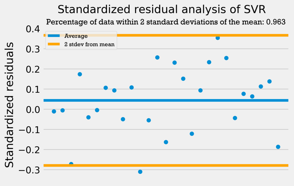
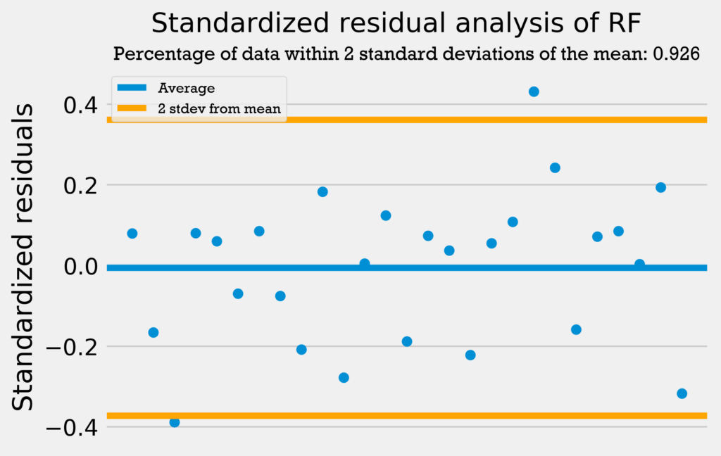
The four graphs below show the standardized residuals for all four models.
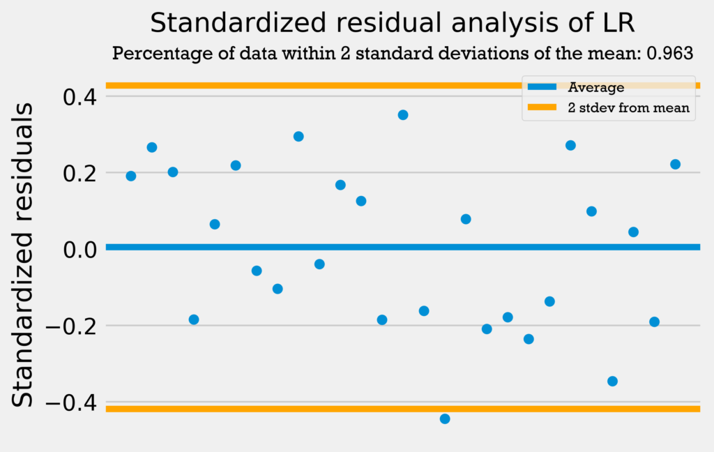
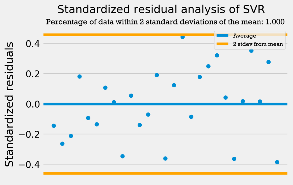
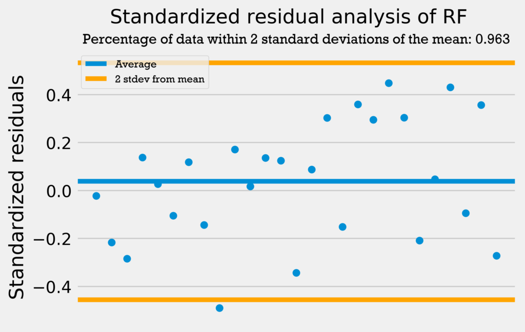
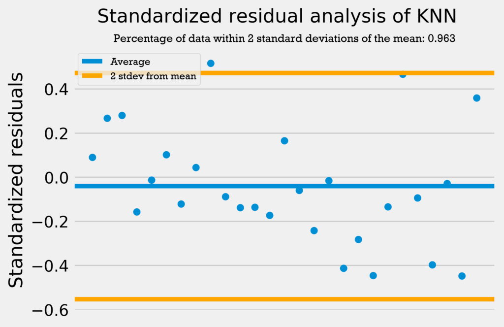
All four models pass the test; they do not have standardized residuals greater than 2 or less than -2, and all models have over 95% of the data within 2 standard deviations of the mean. Therefore, the errors are normally distributed, and the models can be used with no problems.
The standardized residuals test demonstrated that the models’ errors are normally distributed. However, it is still important to test that the models’ errors are random. This means they have no autocorrelation, or that if at one point the model predicts a much higher value than expected, that the next points do not also predict a much higher value.
To test for autocorrelation, I first performed a Durbin-Watson test. A Durbin-Watson test tests for autocorrelation in a regression’s residuals. A DW test statistic of 2 indicates no autocorrelation. A DW test statistic between 0 and 2 indicates positive autocorrelation, and a test statistic between 2 and 4 indicates negative autocorrelation.
The table below shows the DW test results for all four regressions.
| Regression type | DW test statistic |
|---|---|
| Linear | 2.075 |
| Support vector | 1.996 |
| Random forest | 1.943 |
| k-Nearest Neighbors | 1.759 |
Three of the four regressions have a DW test statistic very close to 2, indication no autocorrelation. The k-NN regression has the DW test statistic that is farthest from 2. However, it is very close, at an error of less than 0.25. Therefore, none of the regressions have a significant autocorrelation, and their errors are random.
Lastly, I performed a Jarque-Bera test on the residuals to confirm the residuals’ normality. The null hypothesis of a Jarque-Bera test is that the residuals are normally distributed. A JB value of 0 indicates the residuals are normally distributed (so higher values are worse). Unlike in the simple regressions, where a lower p-value is “better” (because we can reject the null hypothesis that the factors are not related), here a higher p-value is “better”, because it means there is a higher probability the null hypothesis (that the residuals are normally distributed) is more likely to be true.
The table below shows the results of the JB test. Skewness and kurtosis both measure the “tailedness” of a distribution, or how much data is on the ends of the distribution (as opposed to the middle). Skewness measures whether the distribution is skewed to the left (negative skew, and the mean is to the left of the peak) or right (positive skew, and the mean is to the right of the peak). Kurtosis measures how much data is on the ends of the distribution; a positive value indicates heavy-tails (a lot of data in the tails), and a negative value indicates light-tails. A perfect normal distribution has a skewness of 0 and kurtosis of 3.
| Regression type | JB test statistic | p-value | Skewness | Kurtosis |
|---|---|---|---|---|
| Linear | 1.334 | 0.513 | -0.190 | 1.980 |
| Support vector | 0.908 | 0.635 | -0.012 | 2.102 |
| Random forest | 0.889 | 0.641 | -0.152 | 2.165 |
| k-Nearest Neighbors | 0.897 | 0.639 | 0.402 | 2.610 |
Though the JB test statistic is not very close to 0, the high p-values indicate there is a low probability we can reject the null hypothesis that the residuals are in a normal distribution. This is further proven by the skewness being near 0 for all the regressions, and the kurtosis being near 3.
By examining the residuals in a standardized residuals test, Durbin-Watson test, and Jarque-Bera test, we can conclude that the errors in the model are random and normally distributed. Therefore, the models can be used accurately.
Model results: assists
The following four graphs show each model’s predicted assists for the draft class.
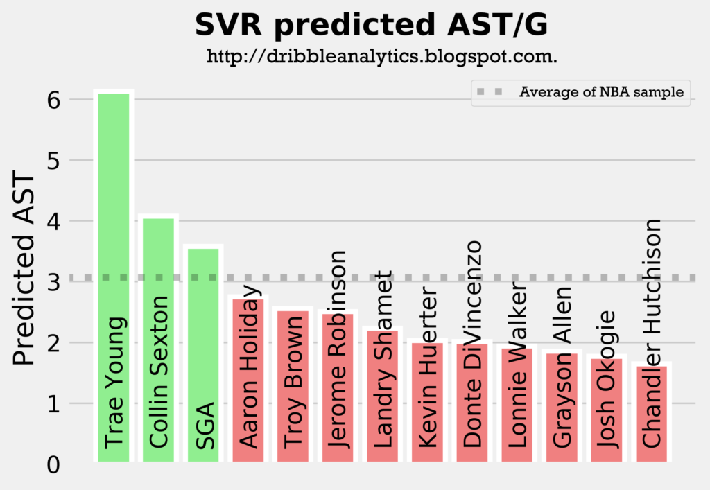
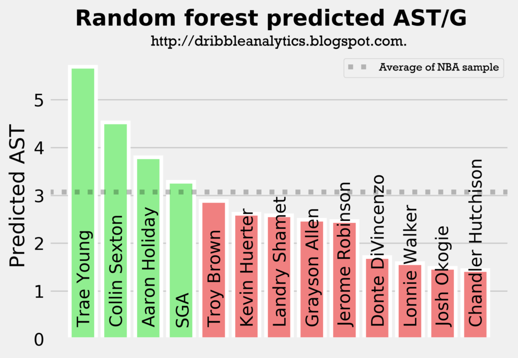
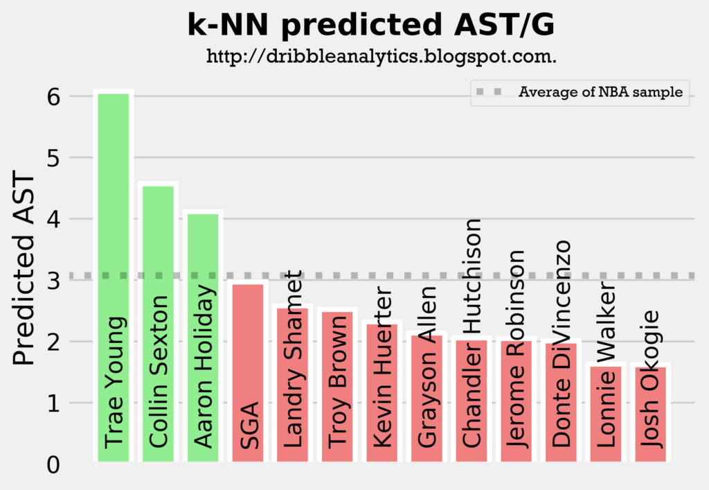
All four models predict Trae Young and Collin Sexton will have the most assists out of all the guards in the draft class, followed by either Aaron Holiday or SGA. This aligns with what we would expect, as these four players are the main pure point guards in the draft.
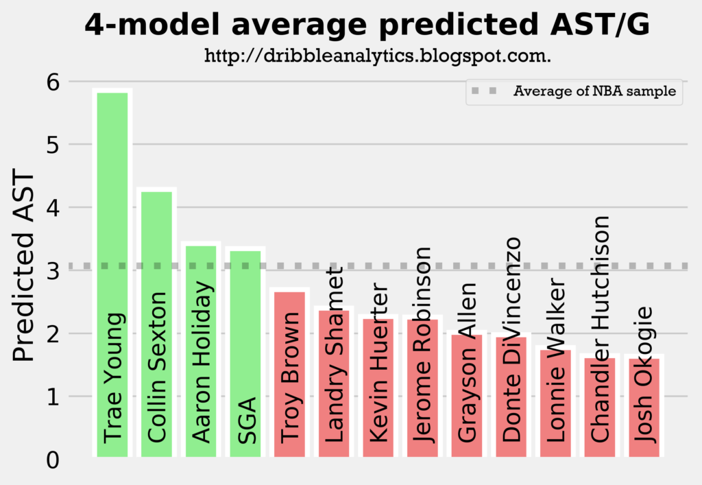
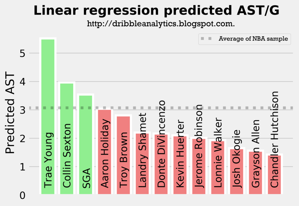
The graph below averages the predicted assists from all four models.

The models all show that Trae Young will be the best facilitator by a decent margin, and that Collin Sexton will be an above-average facilitator. Meanwhile, Holiday and SGA will be at about the sample’s average, and the other guards (all of whom were not drafted to really lead an offense) will have below-average assist totals.
Model accuracy: turnovers
Rsquared, mean squared error, and cross-validation
The two graphs below show the rsquared and mean squared error of the four regressions predicting turnovers.
Though all the rsquareds are low, they are all significantly higher than the rsquared of the simple correlation between college and NBA turnovers.
According to the rsquared and mean squared error results, the linear regression is the most accurate, followed by the support vector regression, k-Nearest Neighbors regression, and random forest regression.
The linear regression had a cross-validation score for explained variance of 0.12, with the 95% confidence interval being +/- 1.20. Though the rsquared is within the 95% confidence interval for explained variance, the broad range and low cross-validation score shows that the model is likely overfitting, and will have high variance on other datasets.
The support vector regression had a cross-validation score of 0.27, with the 95% confidence interval being +/- 0.24. The cross-validation score is lower than the rsquared, but the 95% confidence interval range is not too large. So, it is likely not overfitting.
The random forest regression had a cross-validation score of 0.35, with the 95% confidence interval being +/- 0.72. Unlike the other regressions, the random forest’s cross-validation score was higher than its rsquared. This makes it very unlikely that the model is ovefitting.
The k-Nearest Neighbors regression had a cross-validation of 0.31, with the 95% confidence interval being +/- 0.17. The 95% confidence interval range is the smallest of the four regressions, and the cross-validation score is very close to the rsquared (0.31 vs. 0.36). Therefore, the model is probably not overfitting.
Though the cross-validation scores’ 95% confidence intervals have high ranges, all the rsquareds are within the interval. The linear regression will likely have a very high variance when applied to other datasets (and is likely overfitting to some extent), while the other models will not have this same variance.
Residuals tests
The four graphs below show the standardized residuals for all four models.
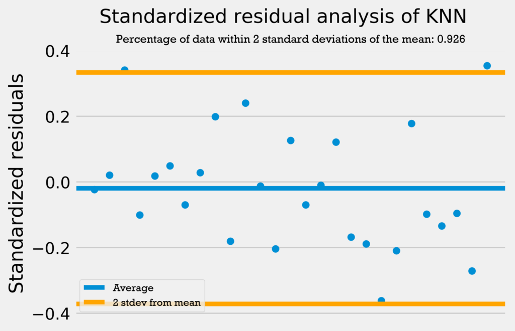
Only the support vector regression has over 95% of its data within 2 standard deviations from the mean. However, the other four regressions are only 1 datapoint away from having 95% of the data within 2 standard deviations from the mean. This combined with the fact that none of the models have a standardized residual above 2 or below -2 demonstrates that the errors are normally distributed and the models can be used with no problems.
The table below shows the Durbin-Watson test results for the four regressions.
| Regression type | DW test statistic |
|---|---|
| Linear | 1.990 |
| Support vector | 1.890 |
| Random forest | 2.031 |
| k-Nearest Neighbors | 2.057 |
All the values are very close to 2, indicating no autocorrelation in the residuals. Therefore, according to the DW test, the errors in the model are random.
The table below shows the Jarque-Bera test results for the four regressions.
| Regression type | JB test statistic | p-value | Skewness | Kurtosis |
|---|---|---|---|---|
| Linear | 0.285 | 0.867 | 0.101 | 2.539 |
| Support vector | 0.660 | 0.719 | -0.330 | 2.610 |
| Random forest | 0.085 | 0.958 | -0.110 | 2.834 |
| k-Nearest Neighbors | 0.817 | 0.665 | 0.378 | 2.608 |
All of the results indicate the residuals are likely normally distributed, especially for the random forest regression. The random forest’s JB test statistic is near 0, and the very high p-value indicates there is a very small probability of rejecting the null hypothesis that the data is normally distributed. Furthermore, the skewness is near 0, and the kurtosis is near 3.
The other three regressions also have encouraging results; their JB test statistic values are low, and their p-values are high. They have minimal skewness and kurtosis very close to 3.
Like in the assists models, the standardized residuals test, Durbin-Watson test, and Jarque-Bera test show that the models’ residuals are random and normally distributed. This means that, like the assist models, the turnover models can be used accurately.
Model results: turnovers
The four graphs below show the predicted turnovers for the 2018 draft class from each of the four models.
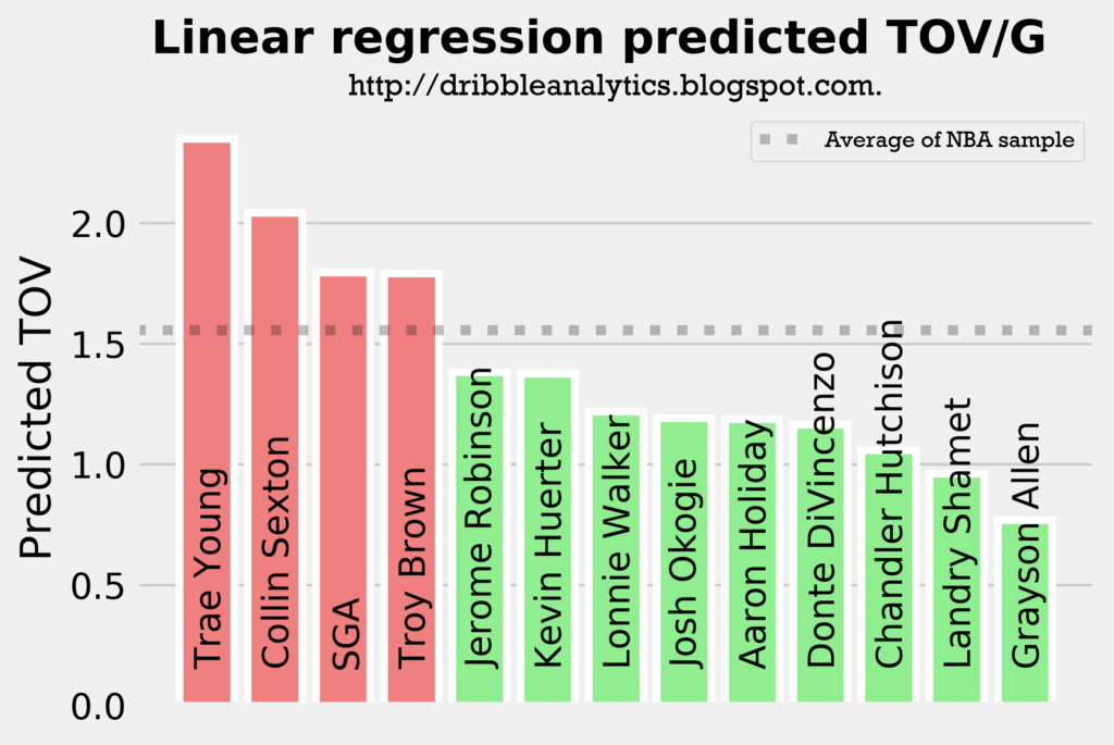
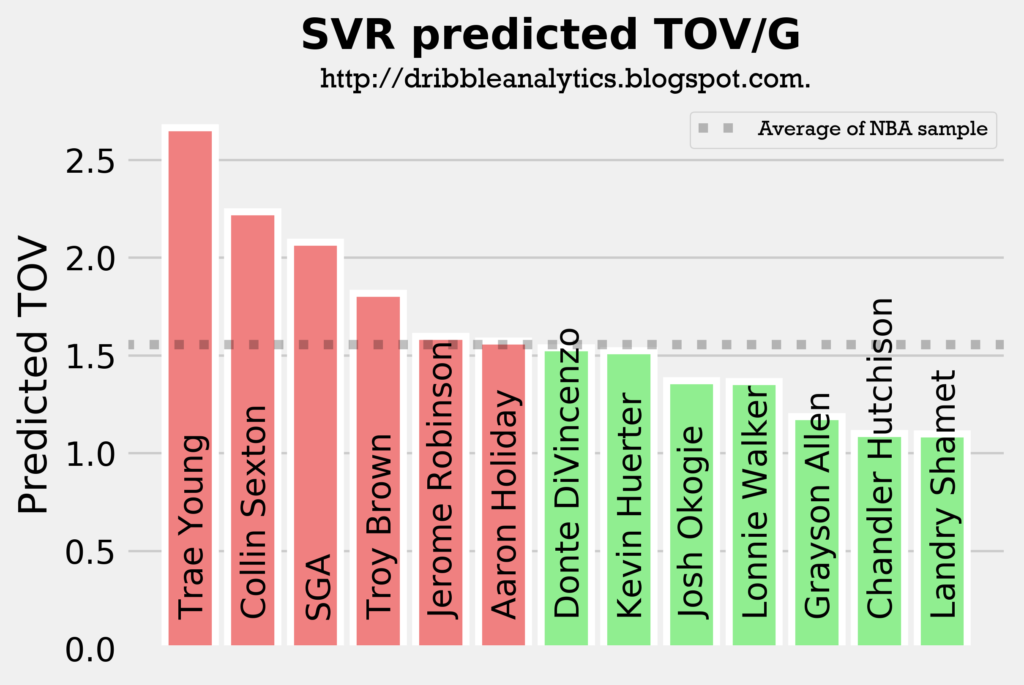
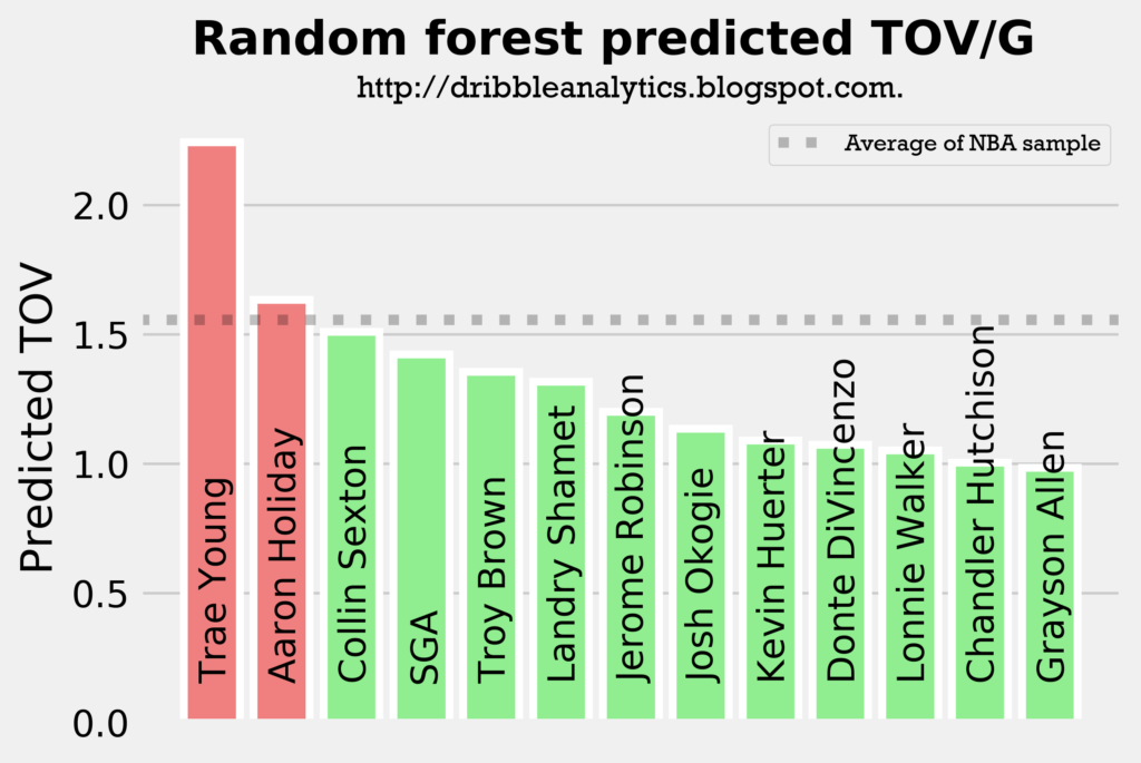
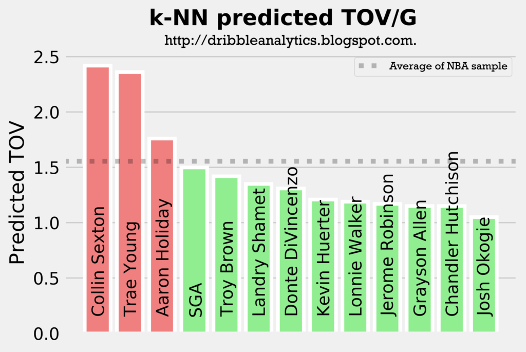
As with the assists models, Trae Young and Collin Sexton are in the top 3 in projected turnovers in all four models. This is expected, however, as they will likely have the highest usage rates and will facilitate the offense. Interestingly, SGA and Aaron Holiday, who are also expected to have sizable facilitating roles have below-average predicted turnovers in a couple of the models.
The graph below shows the average of the predicted turnovers from the four models.
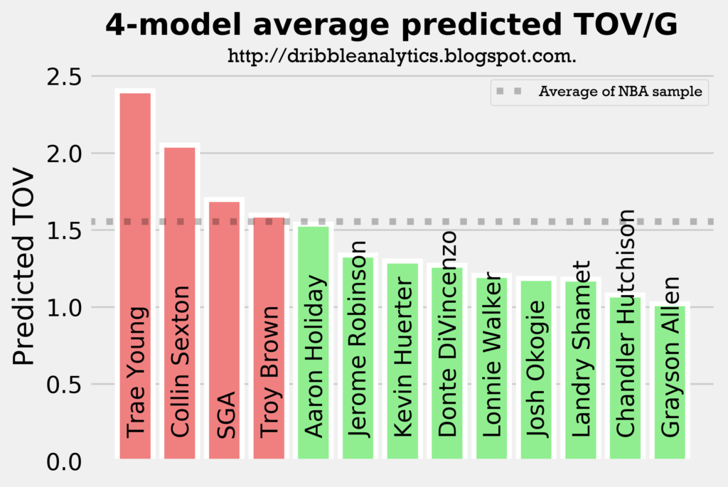
As expected, Trae Young and Collin Sexton placed 1 and 2. However, Troy Brown is surprisingly high, especially given that he is more of a SG/SF combo than a facilitator. So, we wouldn’t expect him to have similar turnover projections to SGA and Aaron Holiday.
Assist to turnover ratio projection
Dividing the average projected assists by the average projected turnovers can give us a projection for assist to turnover ratio. This is important, as it gives context to some of the high projections (such as Trae Young being first in both projected assists and projected turnovers).
The graph below shows the projected assist to turnover ratio.
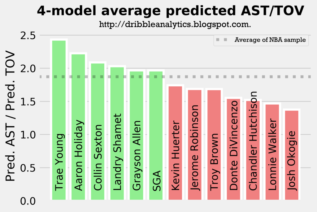
While Trae Young has the highest projected turnovers by a decent margin, he also has the highest projected assist to turnover ratio. Aaron Holiday had a higher projected assist to turnover ratio than Collin Sexton, who had the second highest projected assists. This is because of Holiday’s low turnovers.
Landry Shamet and Grayson Allen also have an above-average projected assist to turnover ratio. Therefore, we can reasonably expect that they’ll be good facilitators in their limited roles (not necessarily creating offense like a traditional point guard, but swinging the ball around/continuing ball movement).
Conclusion
The models predict Trae Young will be the best facilitator in the draft class; he has the highest projected assists by a significant margin, and has the highest projected assist to turnover ratio.
Collin Sexton and Aaron Holiday will likely be the next best facilitators; though Sexton has more projected assists than Holiday, Holiday has a higher projected assist to turnover ratio.
Following the facilitating guards like Young, Sexton, Holiday, and SGA, Landry Shamet and Grayson Allen are projected to be the best facilitators in their limited roles, as they both have an above-average assist to turnover ratio.