Introduction
Following the end of last season, NBA.com released its All-Decade team for the 2010s. The teams consider player performance from the 2009-2010 season until the 2018-19 season.
Given the wide time frame, not every player played the entire decade. Also, some players dropped off at the start of the decade or started their prime at the decade’s end. Beyond LeBron and Durant, there’s no player with constant success throughout the decade. For example, Dwight Howard dominated in the early part of the decade, but fell off. Meanwhile, Giannis wasn’t even drafted until 2013 and only made his first All-NBA team in 2016-17.
This difference in time makes weighting player performance hard. Are several good seasons better than a couple excellent seasons? Or are a couple excellent seasons better than several good seasons? Whichever one we choose results in shuffling the All-Decade team. For the most part, these boundaries of sustained versus peak success are subjective.
To approach this problem in a different way, we will use machine learning.
Methods
The premise
We will approach the problem as follows:
- Create models that predict All-NBA probability within a given season (more discussion of this later)
- Take the sum of All-NBA probabilities for each player throughout the decade
- Organize the teams based off highest probabilities
The above lets us compare different numbers of different level seasons. For example, suppose player 1 earned a 75% All-NBA probability in two seasons. That’s equal to player 2 earning 50% All-NBA probability in three seasons. This lets us reward longevity without penalizing sustained peak performance.
By predicting All-NBA selections, we’re missing one notable thing: playoff performance. There’s no playoff award system we can use to give a bonus to players for their playoff performance. This will hurt players like Kawhi Leonard and Kobe Bryant. Both players won 2 rings in the decade, but only had a few All-NBA level seasons. So, their cumulative All-NBA shares don’t quantify their impact well.
The models: last year
Last year, we used machine learning to predict the All-NBA teams. The models tested well on our historical data set and nailed last year’s teams.
The models correctly predicted the 15 players to make an All-NBA team. Out of these 15 players, 12 were in the correct spots. The 3 misses were tight races that we pointed out might go the other way. They were:
- Damian Lillard over Stephen Curry. The difference between their All-NBA probability was less than 0.001. We pointed out the spot belonged to Curry.
- Joel Embiid over Nikola Jokic. This is the most debated All-NBA selection. Our models gave Embiid a 0.900 probability and Jokic a 0.897 probability. We leaned towards giving Jokic the spot given his team success.
- Kevin Durant over Paul George. This is a case of narrative and defense. The models don’t pick up on excellent defense, so, they underestimated George. Also, the negative narrative surrounding Durant hurt his chances. We pointed out the spot belonged to George.
Altogether, last year’s All-NBA models were almost perfect. Though our models for this problem are different, last year’s success shows us that we can accurately predict All-NBA teams.
The models: now
To give each player an All-NBA score, we’ll create models trained on historical data. We’ll then use the models to predict All-NBA probabilities for every player season from 2009-2010 to 2018-19.
Our data consists of almost every player season since the 1979-1980 season (introduction of the 3-point line). We excluded players who entered the league before 1979-1980. This prevents having players who played part of their careers with the 3-point line and part without it. Though our model inputs are not related to 3-pointers, this gives us some consistency.
In total, we had 15,355 samples in our data set. For these samples, we used the following features (data was collected from Basketball-Reference):
| Play time | Counting stats | Advanced stats |
|---|---|---|
| G | PPG | VORP |
| MP | TRB | WS |
| AST |
These are the most basic indicators of player performance. Though it seems we’re missing a couple things, the models performed well with these inputs. Along with playoff performance, we’re missing:
- Defensive stats. Most players aren’t going to make an All-NBA team just because of defense. Furthermore, among All-NBA players, there’s a broad range of defensive effort. This makes defensive stats mostly random. The models still capture the effect of excellent defense and good offense; win shares reflects this. For example, Rudy Gobert was third in the NBA in win shares last year because of his defense. So, he gets a bonus for being a good defender without us including defensive stats.
- Team success stats. Though team success plays a role in All-NBA selections, and we included it last year, it turns out to not be crucial. A player with incredible stats will make an All-NBA team regardless of their team success. Furthermore, team success relates to player stats in a circular way; better teams have better players.
- Position. Positions aren’t always clear, making it difficult to add a position factor. Instead, we create teams by giving each team 2 guards, 2 wings, and a big. We assign the best remaining player to the highest available spot in his position.
With these 7 features, we created 4 different models:
- Support vector classifier
- Random forest classifier
- K-nearest neighbors classifier
- Gradient boosting classifier
Note that we’re using classification models here. These classify a player as either an All-NBA player (earning a 1) or not an All-NBA player (earning a 0). However, this classification doesn’t give us a lot of information. Instead of using classes, we’ll use the prediction probabilities. This is the probability the model gives for each player to make an All-NBA team. The models classify any player with a probability above 50% as a 1 (All-NBA player).
Using prediction probabilities, we can compare different players. We can also sort the teams, as a higher prediction probability indicates higher All-NBA chances. So, the higher a player’s prediction probability, the higher the slot on the team he earns. This also allows us to create teams by position; we place the player with the highest prediction probability in the correct position for the highest available team. Each team has 2 guards, 2 wings, and a big.
We’ll train these four models on a randomly selected 75% subset of All-NBA data from 1979-1980 until 2008-2009. Then, we’ll predict All-NBA probabilities for the 2009-2010 to 2018-2019 seasons. We’ll sort the probabilities into teams as described above.
Model analysis
The dummy classifier
When evaluating our models, we’ll compare them to the “dummy classifier”. The dummy classifier is a random model. Comparing our models to the dummy classifier contextualizes their performance. This allows us to see if our models a more predictive than a random model.
The dummy classifier generates predictions with respect to the training set’s class distribution. Because our training set has 3.27% All-NBA players, the dummy classifier will randomly predict 3.27% of the test set to make an All-NBA team.
Understanding the data & explaining performance metrics
In any given year, a small percentage of NBA players make an All-NBA team. For classification models, the most basic metric of performance is accuracy. This measures the percentage of correct predictions.
Given the imbalance of the data set, accuracy isn’t useful here. Among our training set (what we use to train the models) of 7,892 player seasons, there were 258 All-NBA seasons. This amounts to 3.27%. The testing set (what we use to test model performance) has a similar imbalance. Among 2,631 player seasons, there were 103 All-NBA seasons, or 3.91%. So, we could “predict” over 95% of players correctly by saying no one will make an All-NBA team.
Given that a model predicting all 0s will have over 95% accuracy, we’ll want to use some other metrics along with accuracy. Two other basic, more useful metrics are precision and recall. Precision measures how often our models correctly predicted a player will make an All-NBA team. Meanwhile, recall measures how many All-NBA players our model found.
Recall is crucial here, as it measures our ability to find All-NBA players. A model predicting all 0s would have high accuracy, but its recall would be 0.
Along with precision and recall, we’ll use a couple other metrics. First, we’ll use F1, which combines precision and recall. This gives us a way to compare two models if one has higher precision, but the other has higher recall. We’ll also consider log loss, which is almost like accuracy, but for prediction probabilities. Log loss tests the uncertainty of our predictions based on how much the prediction probability varies from the actual label (1 or 0). While higher is better in all our other metrics, a lower log loss is better, as it indicates lower uncertainty.
Finally, we’ll also consider the ROC curve and the area under it. The ROC (receiver operating characteristics) curve shows us how well our models differentiate between the two classes.
Note that higher accuracy, precision, recall, and area under ROC is better. The best possible value for these is 1. Meanwhile, lower log loss is better, with a best possible value of 0 (in some cases, log loss of 0 isn’t actually possible, as some models never predict 100% or 0% certainty, so their log loss can only be arbitrarily close to 0).
Cross-validation
One concern when training these models is that they only perform well on a certain split of the data set. We call this overfitting; it occurs when the model learns the training data “too well.” So, while it’s accurate on that one split, it can’t predict other data splits well. To avoid overfitting, we’ll do two things:
- Grid search for hyperparameters. This sounds fancier than it is. Each model has “hyperparameters”, or elements that determine how the model fits the data. In a line, the slope is a hyperparameter. We determined hyperparameters using grid search. This means we created a “grid” of possible hyperparameters. Then, we trained the models on each combination of this “grid.” For each combination, we cross-validated the performance, meaning we tested the performance against different splits of the data. From this, we selected the hyperparameters that resulted in the best performance. For this task, we selected the hyperparameters that resulted in the best recall.
- k-fold cross-validation. We’ll split the data into k bins (3 in this case), use 1 bin as testing data and the other 2 as training data, then test the model. We’ll then repeat this for the other combinations of bins. The average performance gives us an idea of performance across different splits. If our models perform much lower in certain splits, then they’re overfitting.
Confusion matrices
Confusion matrices help us visualize model performance. They show true positives (correctly predicted 1s), true negatives (correctly predicted 0s), false positives (falsely predicted 1s), and false negatives (falsely predicted 0s). The four graphs below are the confusion matrices for our four models.

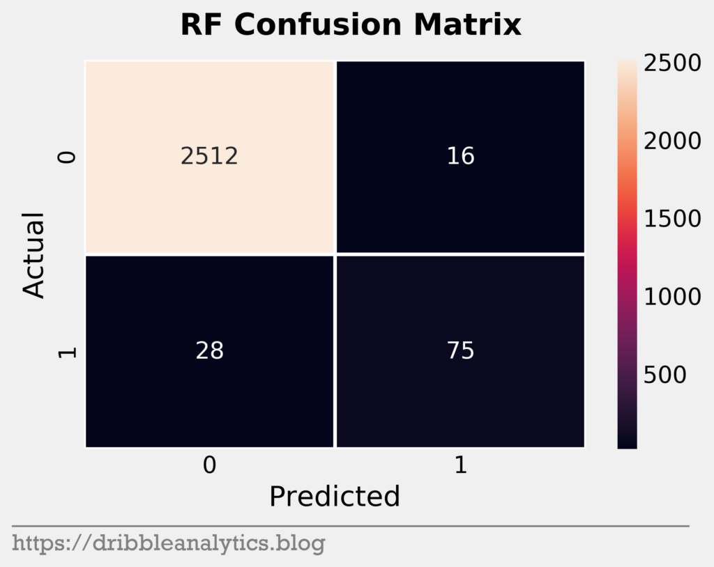


It seems that the models were all similar in their predictions. Given the imbalance of the data set, it’s expected that the models will mostly consist of true negatives. The one noticeable trend here is that the KNN seems stingy with predicting positives, while the GBC seems generous.
Performance metrics
The table below shows the performance metrics for our four models, along with the performance of the dummy classifier (random model).
| Model | Accuracy | Recall | Precision | F1 | Log loss |
|---|---|---|---|---|---|
| SVC | 0.984 | 0.738 | 0.826 | 0.779 | 0.06 |
| RF | 0.983 | 0.728 | 0.824 | 0.773 | 0.04 |
| KNN | 0.984 | 0.66 | 0.895 | 0.76 | 0.184 |
| GBC | 0.982 | 0.777 | 0.769 | 0.773 | 0.05 |
| Dummy | 0.928 | 0.049 | 0.052 | 0.05 | 2.494 |
These scores are quite strong given the imbalance of the data set. To compare each model’s performance to the random model, we’ll take (model performance – random model performance) / (random model performance). The table below shows the improvement for each model.
Because accuracy is at most 1, the highest accuracy improvement above random for any model is 7.76%. So, along with accuracy improvement, we have percentage of possible accuracy improvement.
| Model | Accuracy imp. | % of possible Accuracy imp. | Recall imp. | Precision imp. | F1 imp. | Log loss imp. |
|---|---|---|---|---|---|---|
| SVC | 6.03% | 77.78% | 1406.12% | 1488.46% | 1458.00% | 97.59% |
| RF | 5.93% | 76.39% | 1385.71% | 1484.62% | 1446.00% | 98.40% |
| KNN | 6.03% | 77.78% | 1246.94% | 1621.15% | 1420.00% | 92.62% |
| GBC | 5.82% | 75.00% | 1485.71% | 1378.85% | 1446.00% | 98.00% |
All the models have a significant improvement over random. They are all cover at least 75% of the possible accuracy improvement. Furthermore, they all have better precision, recall, and F1. The log loss improvement scores are actually negative, as the model log loss is lower than the random log loss. We translated them to positive improvement. Those improvement scores are also impressive given that the highest possible improvement is 100% (if log loss was 0, then (0 – random log loss) / (random log loss) = 1).
Now, we’ll look at the ROC curves. The graph below shows the ROC curves for the four models.
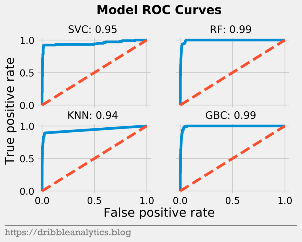
Each model has a near-perfect area under ROC curve. The sharp curve indicates a strong ability to differentiate between classes.
Lastly, we’ll look at the cross-validated scores for accuracy and recall, along with their confidence intervals. If the cross-validated scores are close to our real scores, then our models are probably not overfitting. The table below shows the cross-validated scores for each model.
| Model | Normal accuracy | CV accuracy | 95% confidence interval | Normal recall | CV recall | 95% confidence interval |
|---|---|---|---|---|---|---|
| SVC | 0.984 | 0.983 | +/- 0.004 | 0.738 | 0.777 | +/- 0.068 |
| RF | 0.983 | 0.984 | +/- 0.008 | 0.728 | 0.739 | +/- 0.118 |
| KNN | 0.984 | 0.982 | +/- 0.001 | 0.66 | 0.651 | +/- 0.115 |
| GBC | 0.982 | 0.983 | +/- 0.008 | 0.777 | 0.748 | +/- 0.092 |
All the models have cross-validated scores close to their real ones. Some even have higher cross-validated scores, indicating they perform even better on other splits on the data. The recall scores have wider confidence intervals because the small positive class size means that a few different predictions affect recall much more than accuracy.
Given all the performance metrics above, we’re inclined to think our models are strong indicators of All-NBA performance.
Results
To create the All-Decade teams, we’ll use cumulative prediction probabilities from each model. So, we’ll sum each player’s All-NBA probability in each year throughout the decade. This means the highest possible score is 10, which would occur if a player had 100% All-NBA probability every year.
We’ll create the teams by assigning the player with the highest possible score to the highest available slot in his position. For non-obvious positions, we chose the listed player position at the player’s most recent All-NBA selection. So, Kevin Love, Blake Griffin, and LaMarcus Aldridge (the main players who’d have this problem) are all forwards.
We also included the five players with the highest totals – regardless of position – who missed the teams (shown in the last row of each table). The four tables below show each model’s All-Decade teams.
| SVC | Guard | Guard | Forward | Forward | Center |
|---|---|---|---|---|---|
| 1st team | Russell Westbrook (6.441) | James Harden (6.427) | LeBron James (9.040) | Kevin Durant (8.726) | Anthony Davis (3.850) |
| 2nd team | Stephen Curry (6.263) | Chris Paul (4.667) | Kevin Love (3.482) | Giannis Antetokounmpo (3.000) | DeMarcus Cousins (3.790) |
| 3rd team | Damian Lillard (3.412) | Dwyane Wade (2.569) | Kawhi Leonard (2.538) | Blake Griffin (2.517) | Karl-Anthony Towns (2.990) |
| Just missed | Kyrie Irving (2.561) | Nikola Jokic (2.249) | Dwight Howard (1.930) | Joel Embiid (1.905) | Dirk Nowitzki (1.741) |
| RF | Guard | Guard | Forward | Forward | Center |
|---|---|---|---|---|---|
| 1st team | James Harden (6.554) | Chris Paul (5.326) | LeBron James (8.537) | Kevin Durant (7.554) | Anthony Davis (3.680) |
| 2nd team | Russell Westbrook (5.309) | Stephen Curry (5.246) | Blake Griffin (3.297) | Kevin Love (2.989) | DeMarcus Cousins (2.314) |
| 3rd team | Damian Lillard (3.537) | Dwyane Wade (2.469) | Giannis Antetokounmpo (2.651) | LaMarcus Aldridge (2.651) | Dwight Howard (2.177) |
| Just missed | Carmelo Anthony (2.549) | Dirk Nowitzki (2.326) | Kyrie Irving (2.229) | Paul George (2.223) | Kobe Bryant (2.194) |
| KNN | Guard | Guard | Forward | Forward | Center |
|---|---|---|---|---|---|
| 1st team | James Harden (6.812) | Russell Westbrook (6.153) | LeBron James (8.943) | Kevin Durant (7.082) | Anthony Davis (4.252) |
| 2nd team | Stephen Curry (5.674) | Chris Paul (4.005) | Kevin Love (3.268) | Giannis Antetokounmpo (3.000) | DeMarcus Cousins (2.775) |
| 3rd team | Damian Lillard (3.884) | Dwyane Wade (2.731) | Blake Griffin (2.512) | Carmelo Anthony (2.337) | Karl-Anthony Towns (2.403) |
| Just missed | Kyrie Irving (2.465) | LaMarcus Aldridge (2.270) | Kawhi Leonard (2.214) | Jimmy Butler (2.054) | Paul George (1.972) |
| GBC | Guard | Guard | Forward | Forward | Center |
|---|---|---|---|---|---|
| 1st team | Chris Paul (7.774) | Russell Westbrook (7.408) | LeBron James (9.474) | Kevin Durant (8.085) | Anthony Davis (4.441) |
| 2nd team | James Harden (6.869) | Stephen Curry (6.374) | LaMarcus Aldridge (3.413) | Kevin Love (3.290) | Karl-Anthony Towns (2.678) |
| 3rd team | Damian Lillard (4.128) | Dwyane Wade (2.810) | Blake Griffin (2.948) | Giannis Antetokounmpo (2.876) | DeMarcus Cousins (2.542) |
| Just missed | Paul George (2.481) | Deron Williams (2.446) | Kyle Lowry (2.370) | Dirk Nowitzki (2.358) | Kawhi Leonard (2.272) |
The table below shows the average of the four models.
| Average | Guard | Guard | Forward | Forward | Center |
|---|---|---|---|---|---|
| 1st team | James Harden (6.665) | Russell Westbrook (6.328) | LeBron James (8.998) | Kevin Durant (7.862) | Anthony Davis (4.056) |
| 2nd team | Stephen Curry (5.889) | Chris Paul (5.443) | Kevin Love (3.257) | Giannis Antetokounmpo (2.882) | DeMarcus Cousins (2.855) |
| 3rd team | Damian Lillard (3.740) | Dwyane Wade (2.644) | Blake Griffin (2.819) | LaMarcus Aldridge (2.382) | Karl-Anthony Towns (2.559) |
| Just missed | Kyrie Irving (2.346) | Kawhi Leonard (2.217) | Carmelo Anthony (2.196) | Dirk Nowitzki (1.967) | Paul George (1.948) |
Discussion of results
As expected, LeBron and Durant are a tier above everyone else. They were the two highest scorers in every model. Durant’s score – and the gap between him and the rest of the non-LeBron players – would be even higher had he not gotten injured in the 2014-15 season.
All four models had Harden, Westbrook, Curry, and Paul after LeBron and Durant. These 4 guards composed the first and second team slots in all four models. Curry had the lowest total of the four because of injuries in the 2017-18 and 2018-19 seasons.
Despite only entering the league in 2012 and earning his first All-NBA level selection in 2014, Anthony Davis secured the first team center slot in all four models. This speaks volumes about the weakness of the center position. His competition had durability issues; Dwight Howard dominated early, but fell off after the 2010-2011 season. Similarly, Karl-Anthony Towns only entered the league in 2015. Finally, DeMarcus Cousins myriad of recent injuries prevented him from achieving consistent success.
As mentioned earlier, playoff success is not a factor in these models. While this hurts players like Kawhi and Kobe, this helps a player like Cousins. Cousins puts up excellent counting stats, but a lack of playoff success hurts his reputation.
As an additional interesting thing, we’ll look at the highest individual season All-NBA scores. This isn’t super informative, given that there were 26 seasons with an average All-NBA score over 95%. Any season over a certain threshold is essentially an All-NBA lock. So, the difference between these 26 player seasons is small. However, it still shows some dominant seasons. The table below shows the highest individual season scores. Note that the given year is the year at the start of the season (so 2018 implies the 2018-19 season).
| Maximum | Guard | Guard | Forward | Forward | Center |
|---|---|---|---|---|---|
| 1st team | James Harden, 2014 (0.986) | James Harden, 2016 (0.986) | Kevin Durant, 2013 (0.995) | LeBron James, 2013 (0.990) | Anthony Davis, 2016 (0.934) |
| 2nd team | Russell Westbrook, 2015 (0.982) | James Harden, 2013 (0.971) | LeBron James, 2017 (0.984) | Kevin Love, 2013 (0.980) | Nikola Jokic, 2018 (0.911) |
| 3rd team | Dwyane Wade, 2010 (0.970) | Stephen Curry, 2013 (0.968) | LeBron James, 2015 (0.980) | Jimmy Butler, 2016 (0.977) | Karl-Anthony Towns, 2017 (0.886) |
| Just missed | Kevin Durant, 2009 (0.975) | LeBron James, 2012 (0.974) | Kevin Durant, 2012 (0.974) | LeBron James, 2010 (0.969) | Giannis Antetokounmpo, 2017 (0.967) |
As we’d expect, the table has a lot of LeBron and Durant. 8 of the 20 seasons above come from one of the two players. This number may even be higher if we didn’t need to include centers. The first center (Anthony Davis) came in at the 31st highest total, behind several other LeBron, Durant, Curry, Harden, and Giannis seasons.
Interestingly, Harden has the highest All-NBA scores for 2014 and 2016. However, he won MVP in neither of these seasons. His MVP-winning 2017-18 season isn’t on this list. However, this is in no way a metric for who deserves each MVP, given that there are way more All-NBA players (15) than MVPs (1) in any year. Therefore, the difference between All-NBA probability is small. So, some amazing seasons are missing (like Curry’s unanimous MVP) because they’re just barely lower than some seasons on this list.
Individual player results
To look at annual or cumulative All-NBA shares for any player, click the link below to see an interactive dashboard. This lets you compare any two players over any time frame by their annual or cumulative scores. The link is:
https://dribbleanalytics.shinyapps.io/all-decade-teams/
Conclusion
By taking cumulative All-NBA probability, we can create All-Decade teams. Though they miss the factor of playoff success, the models are strong. Together, they give a complete and objective picture of the best players in the past decade.