There is a summary at the bottom if you want to skip to the results.
Introduction
Last year, media members unanimously selected LeBron James to the All-NBA first team, giving him a record 12 All-NBA first team selections. However, given the Lakers recent struggles and LeBron’s absence earlier in the season, LeBron might miss not only the first team but also the second team. This would mark the first time since his rookie year he misses both of the top two teams.
With two MVP-caliber forwards in Giannis Antetokounmpo and Paul George and two more superstar forwards on top teams in Kevin Durant and Kawhi Leonard, LeBron presents almost no case to earn a spot on the first or second team. Barring a scorching hot run by the Lakers to end the year, LeBron will have a significantly worse team record and worse stats than these 4 players.
For the second year in a row, voters unanimously placed James Harden on the first team. This streak seems certain to extend given Harden’s unreal stats, which put him in a close race with Giannis for the MVP.
Past these certainties, the rest of the All-NBA teams seem up in the air, with close battles in several spots.
Now that we’re just past the All-Star break, the landscape is becoming more clear. To predict the All-NBA teams, I created various classification models.
Methods
Unlike predicting MVP vote share, which is a regression problem, predicting All-NBA teams is a classification problem. The models don’t predict a number such as vote share; instead, they predict a number which represents a “class.” In this case, they classify players as a 1 (All-NBA) or 0 (not All-NBA).
The models also return a probability for these predictions. We can think of these as a certainty of sorts; a player with a 1.0 probability (100%) is a lock to make an All-NBA team.
Because each All-NBA team has 5 players – 2 guards, 2 forwards, and 1 big – I made 1 positive class and used the prediction probability function. Because I can’t teach the models to predict 5 players for each team and to have the predictions follow the positional restrictions, prediction probabilities give more insight than the classes themselves. So, I looked at the prediction probabilities for each player, sorted them by the highest probability (i.e. most certain to make an All-NBA team), and fit the teams accordingly.
Therefore, I made the teams by looking at the prediction probability and assigning the highest probability player to the highest available slot in his position.
Because the majority of All-NBA players also made the All-Star team, my data set consists of every player who played in the All-Star game or made an All-NBA team in each year. Players who were selected as All-Stars, did not play in the game, and were then selected to an All-NBA team were considered in the data set. However, players who were selected as All-Stars, did not play in the game, and then did not make an All-NBA team were excluded for convenience.
I collected the following stats for players who met these restrictions starting with the 1979-1980 season (the introduction of the 3-point line):
| Counting stats | Advanced stats | Team stats |
|---|---|---|
| G | WS | Wins |
| MPG | WS/48 | Overall seed |
| PTS/G | VORP | |
| TRB/G | BPM | |
| AST/G | ||
| STL/G | ||
| BLK/G | ||
| FG% | ||
| 3P% | ||
| FT% |
In total, the data set consisted of 956 players.
Out of the above stats, the following were used as parameters for the models:
| Counting stats | Advanced stats | Team stats | Other |
|---|---|---|---|
| PTS/G | VORP | Wins | All-Star * |
| TRB/G | WS | Overall seed | |
| AST/G | |||
| FG% |
* All-Star = 1 the player was on an All-Star team, 0 = not selected to an All-Star team. This is called a categorical predictor.
I ignored defensive stats (steals and blocks) for 2 reasons:
- Defensive stats are very random in nature. Furthermore, publicly available stats fail to quantify defense. This means they will likely add noise to the models.
- Usually, only big men make an All-NBA team primarily because of defense. These big men will also likely be at least average on offense, post near the best rebound numbers in the league, support good teams. Lastly, their excellent defense will be reflected in their VORP and WS. For example, Rudy Gobert has the third highest WS in the NBA.
I created four classification models:
- Support vector classifier (SVC)
- Random forest classifier (RF)
- k-nearest neighbors classifier (KNN)
- Multi-layer perceptron classifier (or deep neural network, DNN)
Understanding the data
As with all classification models, it’s very important to understand the data. For example, a model may appear very “accurate” by predicting all 0s on a test set if the data mostly consists of 0s.
Out of the 956 data points, 921 were All-Stars, meaning that only 35 out of 956 players made an All-NBA team after not being selected as an All-Star. This comes out to only 3.66%.
525 players made an All-NBA team, or 54.9% of the data set. Consequently, 431 players did not make an All-NBA team, or 45.1%. From a model evaluation perspective, this balance lets us use contextualize a model’s metrics. If a model is accurate on this balanced data set, it is likely a strong model.
Though this isn’t necessary for understanding the data in the context of the model, let’s look at how All-NBA players’ stats differ from the rest of the data set. To do so, we’ll plot a few different relationships and see if there’s a noticeable trend on the graph that separates All-NBA players from non-All-NBA players.
First, let’s look at the relationship between points per game and team wins.
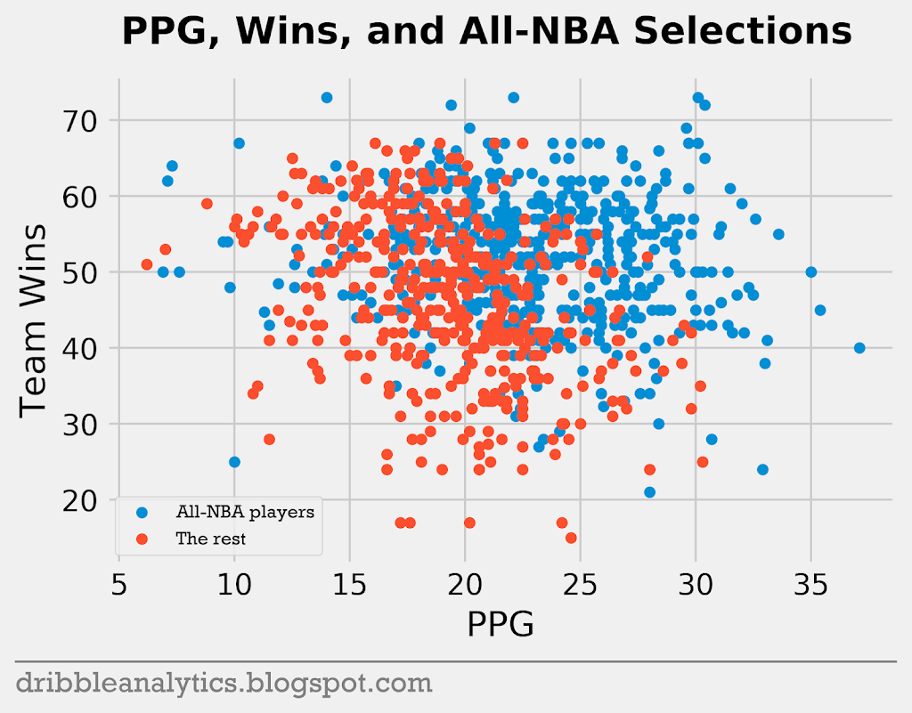
The data seems pretty noisy. In general, it seems that the best scorers will make an All-NBA team more often than contributors on the best team. The relationship between VORP and wins shows a similar phenomenon.
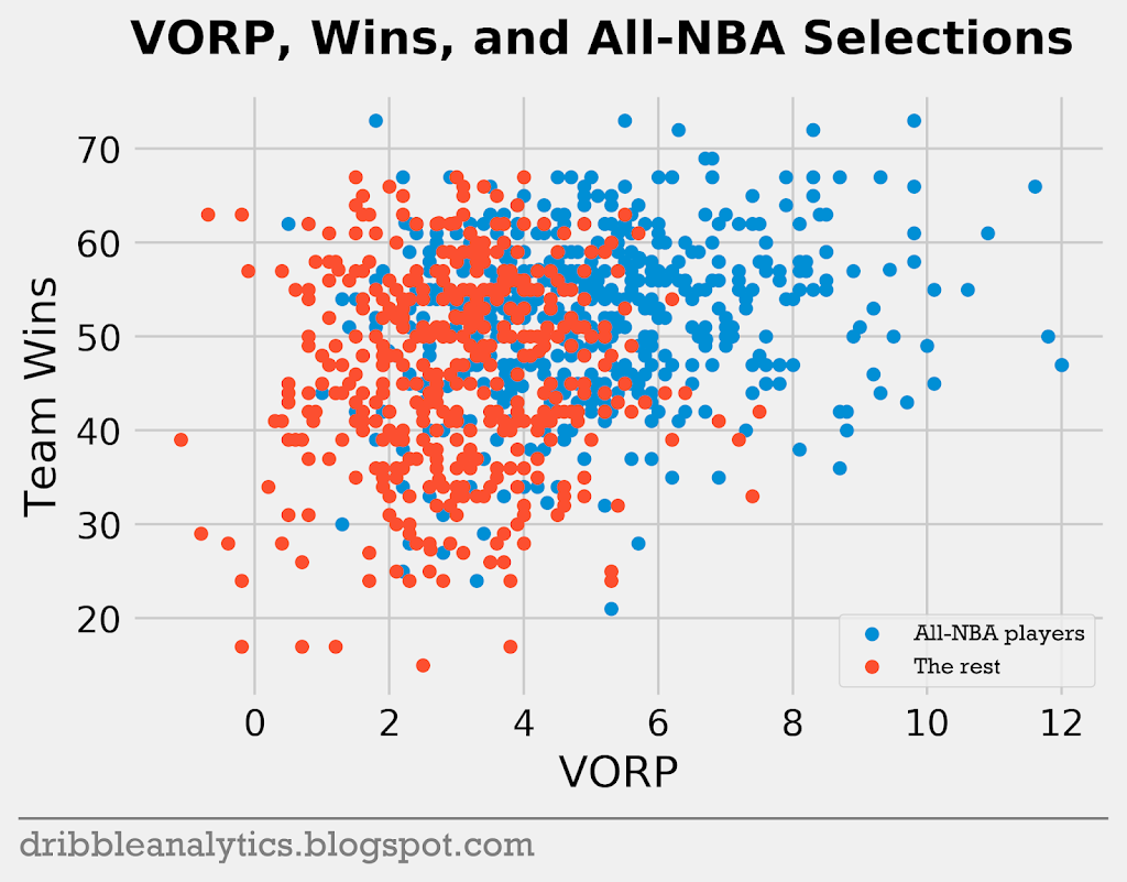
VORP further proves this point that the best players will generally make an All-NBA team regardless of their team success.
Let’s look at how points per game and VORP relate to win shares. Theoretically, the data should become more clear; while win shares depend on team wins, they should isolate each player’s contribution.
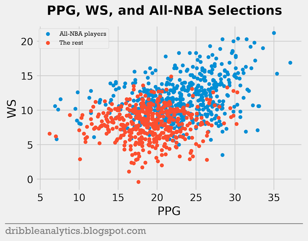
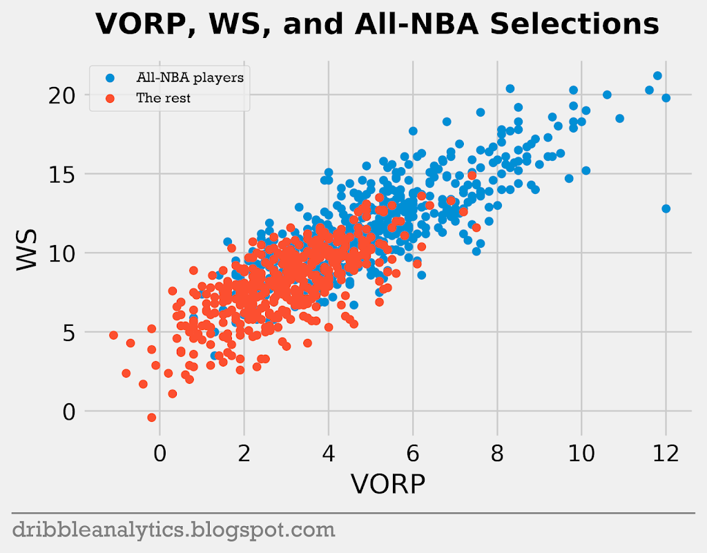
As expected, both relationships have a more common trend, and the data appears more linear when the y-axis is win shares (compared to the lack of a trend when the y-axis was wins). Because win shares try to isolate how much a player contributes, the relationship becomes clear. This drops all the players who served as great role players on excellent teams to the rest of the pack. Now, unlike the team wins relationships, the concentration of All-NBA players always increases as you approach the top right of the graph.
The four graphs below are histograms of each of the 4 stats (PPG, VORP, Team wins, WS) used previously.
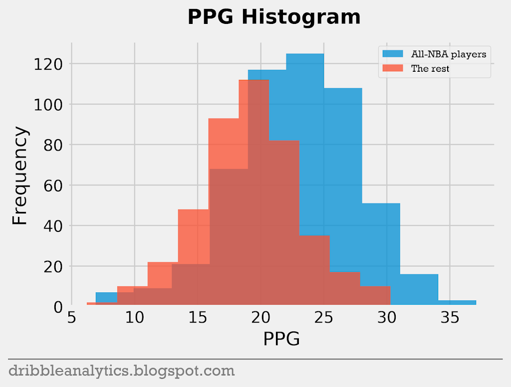
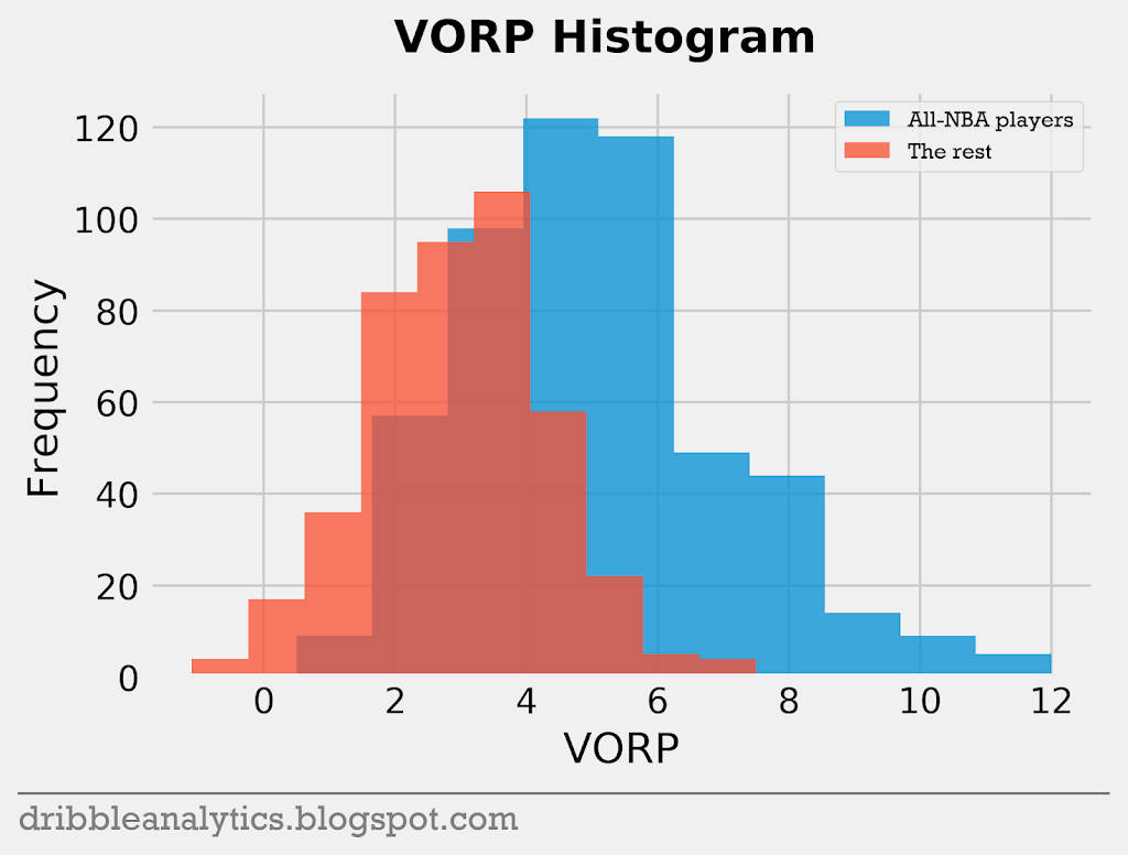
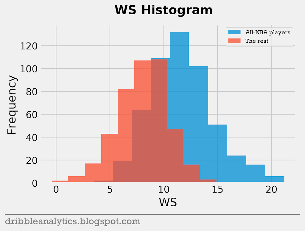
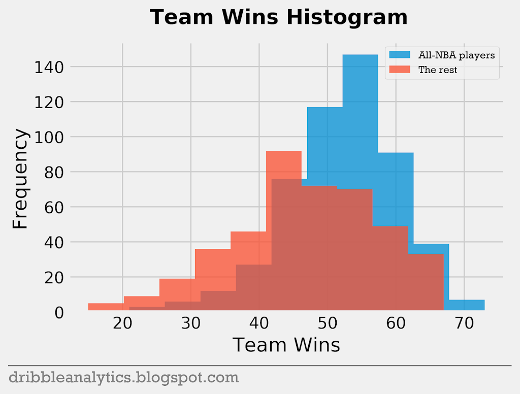
The histograms show that the difference between All-NBA and non-All-NBA players in team wins is small compared to the difference between them in PPG, VORP, and WS. WS seems to show the biggest difference between the two groups of players.
Remember that none of these relationships are important to the models – they’re just interesting to examine.
Model analysis
Basic goodness-of-fit
In evaluating a classification model, the simplest measure of strength is the accuracy score, which measures what percent of the test data the model classified correctly. When we have highly skewed data, accuracy is not a valid indicator of a good model. However, given the balance of the data, accuracy gives us a sense of a model’s strength.
Along with the accuracy score, metrics such as recall, precision, and F1 can give us a sense of a model’s prediction ability. While accuracy just measures correct predictions (accuracy = # of correct predictions / # of data points), these other metrics look at the correct and incorrect predictions differently.
Note that a false positive (FP) occurs when the model predicts a point’s class to be 1 (positive) but the real value is 0 (negative). A false negative (FN) is the opposite; the model predicts a 0 (negative) but the real value is 1 (positive). True positives (TP) and true negatives (TN) occur when the models correctly assign the data to the positive or negative class.
Recall essentially measures a model’s ability to predict the positive class. Recall = TP / (TP + FN), meaning that a “perfect” model that corrects every positive class correctly will have a recall of 1.
Precision does the opposite of recall; it measures the model’s ability to limit false positives. Precision = TP / (TP + FP). The best possible precision score is 1.
F1 combines precision and recall; it equals 2(precision * recall) / (precision + recall). This helps us determine which model is better between two models if one has a higher precision but lower recall. Like recall and precision, F1 values are between 0 and 1, with 1 being the best.
Now that we’re familiar with some of the classification metrics, let’s see how the models fare. The table below shows the scores of all four models on the previously mentioned tests.
| Model | Accuracy | Recall | Precision | F1 |
|---|---|---|---|---|
| SVC | 0.837 | 0.85 | 0.844 | 0.847 |
| RF | 0.808 | 0.819 | 0.819 | 0.819 |
| KNN | 0.803 | 0.772 | 0.845 | 0.807 |
| DNN | 0.808 | 0.819 | 0.819 | 0.819 |
The SVC scores highest in every metric, indicating that it’s probably the best model. The RF and DNN have identical scores in each metric. While the KNN has the lowest accuracy, recall, and F1 score, it has the highest precision score. Given that we’re more interested in the model’s ability to predict the positive class (All-NBA players), the KNN is still very strong.
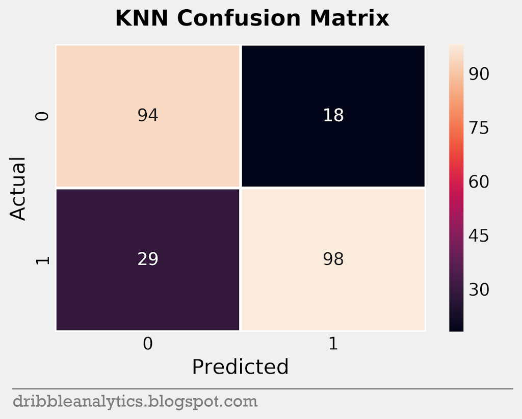
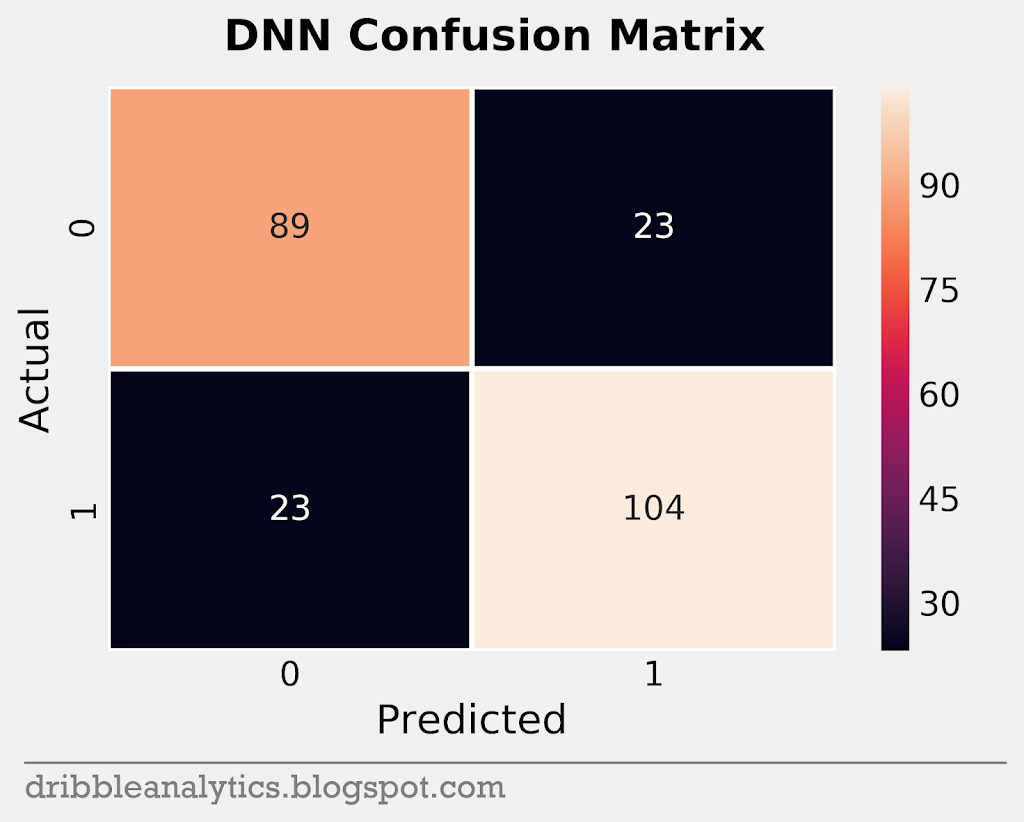
Confusion matrices
A confusion matrix helps visualize a model’s accuracy. The matrix plots the predicted vs. actual classes for each model. So, it plots each model’s true positives (bottom right), true negatives (top left), false positives (top right), and false negatives (bottom left).
In total, the test set had 239 data points. Through the matrices, we’ll understand how the models predicted these points. Below are the confusion matrices for all four models.


Cross-validation
As always, we want to cross-validate the models to ensure they didn’t learn well only for this specific split of data (or, they overfit). With classification models, this is especially important given that the test set could have consisted of mostly one class. Therefore, testing the models’ accuracy scores on different splits will help us determine if they’re overfitting.
The table below shows the cross-validated scores (k = 3) for accuracy and the 95% confidence intervals for these scores.
| Model | CV r-squared | 95% confidence interval |
|---|---|---|
| SVM | 0.766 | +/- 0.081 |
| RF | 0.766 | +/- 0.1 |
| KNN | 0.783 | +/- 0.075 |
| DNN | 0.728 | +/- 0.027 |
None of the models have a cross-validated accuracy score that’s significantly lower than the real accuracy score. This combined with the small confidence intervals implies that it’s unlikely the models are overfitting.
Log loss and ROC curve
The final two metrics we’ll use to evaluate the models are log loss and the ROC curve.
Log loss is like accuracy, but instead of analyzing the labeled predictions, it analyzes the prediction probabilities. This is particularly important given that we’re more interested in the probabilities than we are in the actual labels. A “perfect” model will have a log loss of 0.
The table below shows each model’s log loss.
| Model | Log loss |
|---|---|
| SVC | 0.416 |
| RF | 0.416 |
| KNN | 0.403 |
| DNN | 0.43 |
The SVC and RF have the same log loss, while the KNN has the lowest.
Next, let’s look at the receiver operating characteristics (ROC) curve. The ROC curve plots the true positive rate against the false positive rate. This essentially determines the “separation” between the true positives and true negative. The area under this curve can give us this measure of separation numerically.
If there was no overlap in probability between the true positives and true negatives – meaning the model is “perfect” – the ROC curve would make a right angle, giving us an area under the curve (AUC) of 1. As the overlap increases, the curve gets closer and closer to a 45-degree line (y = x).
Below are the ROC curves and the area under each of them for each of the four models.
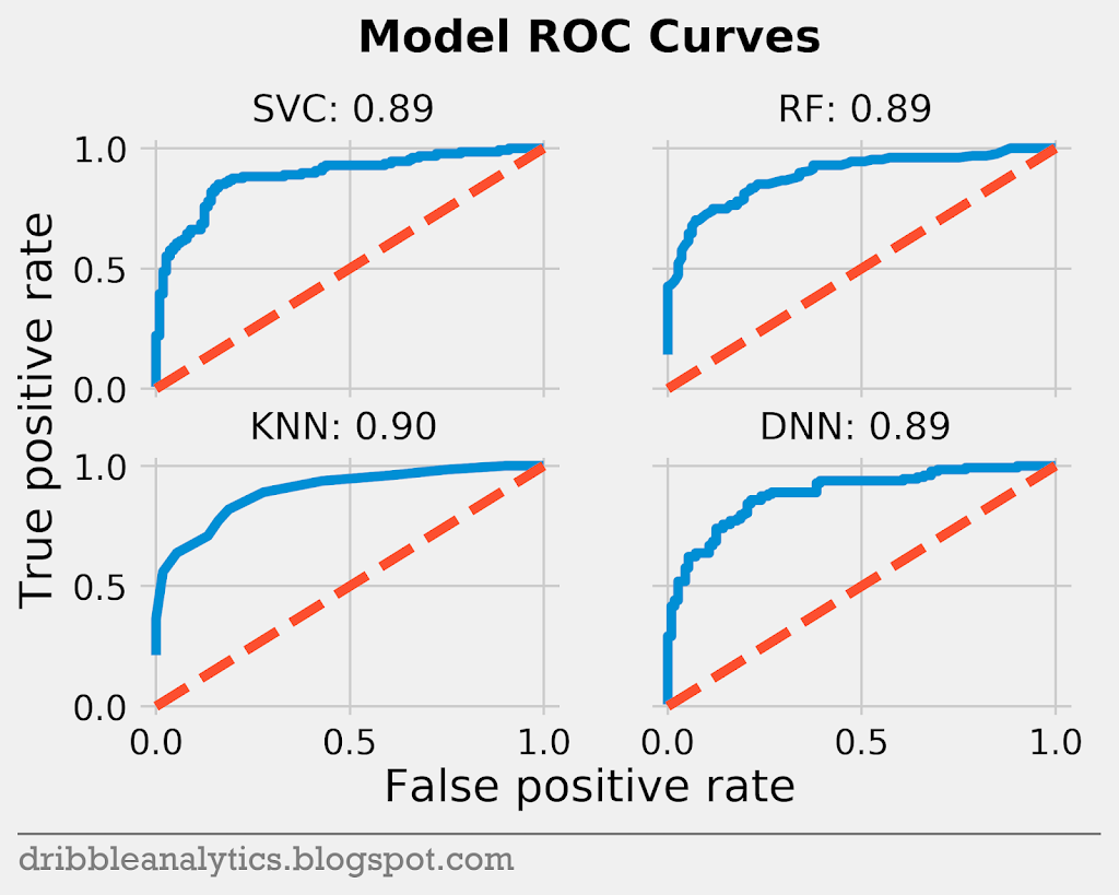
Each of the four models has a similar ROC curve and a near-identical AUC.
Results
As mentioned in the “methods” section, the teams were determined by looking at the prediction probabilities and assigned the highest probability to the highest available slot for that position. In many cases, players have probabilities that are close to equal, meaning their slots are interchangeable and will likely depend on narrative.
Unlike the MVP race, All-NBA teams don’t rely on narrative. Voters don’t experience “fatigue” from voting the same dominant player to the first team every year; typically, the best players make it. When the difference between probabilities is negligible, these factors may come in to play.
The prediction data set consists of every player who played in the All-Star game and Rudy Gobert. Gobert was included given that he’s considered the biggest snub, has excellent advanced stats, and holds the “defensive anchor” quality that has lead others such as DeAndre Jordan to All-NBA selections.
The data was collected during the All-Star break and certain stats (team wins, win shares, etc.) were scaled up to an 82-game season.
In previous years, LaMarcus Aldridge has made an All-NBA team as a forward. However, this year, Aldridge has played over 90% of his minutes at center, the highest mark since his rookie season by a large margin. Therefore, he is considered a center. Anthony Davis is also considered a center, as he plays more than 95% of his minutes at center. Davis’s predictions are also much higher than his real chances, given that the models don’t know about his current situation.
Below are the predictions for each of the four models. In parentheses after each player’s name is their prediction probability, or the model’s certainty that the player will make an All-NBA team. The value is rounded to three decimal places unless the model returned it with fewer than three decimal places. An asterisk after a player’s name indicates that the player has identical prediction probabilities to another player who has the same number of asterisks after his name.
| SVC Predictions | Guard | Guard | Forward | Forward | Center |
|---|---|---|---|---|---|
| 1st team | Stephen Curry (0.991) | James Harden (1.000) | Giannis Antetokounmpo (1.000) | Kevin Durant (0.996) | Joel Embiid (0.990) |
| 2nd team | Damian Lillard (0.961) | Russell Westbrook (0.961 | Paul George (0.995) | Kawhi Leonard (0.954) | Nikola Jokic (0.978) |
| 3rd team | Kyrie Irving (0.891) | Ben Simmons (0.564) | LeBron James (0.730) | Blake Griffin (0.462) | Rudy Gobert (0.935) |
| RF Predictions | Guard | Guard | Forward | Forward | Center |
|---|---|---|---|---|---|
| 1st team | Stephen Curry (0.94) * | James Harden (1.0) | Paul George (1.0) | Giannis Antetokounmpo (1.0) | Nikola Jokic (0.9) |
| 2nd team | Damian Lillard (0.94) * | Russell Westbrook (0.73) | Kevin Durant (0.99) | Kawhi Leonard (0.67) | Rudy Gobert (0.85) |
| 3rd team | Kyrie Irving (0.65) | Kemba Walker (0.44) | LeBron James (0.66) | Blake Griffin (0.39) | Joel Embiid (0.82) |
| KNN Predictions | Guard | Guard | Forward | Forward | Center |
|---|---|---|---|---|---|
| 1st team | Stephen Curry (1.0) | James Harden (1.0) | Paul George (1.0) * | Giannis Antetokounmpo (1.0) * | Nikola Jokic (0.917) ** |
| 2nd team | Damian Lillard (0.75) | Kyrie Irving (0.75) | Kevin Durant (1.0) * | Kawhi Leonard (0.917) | Joel Embiid (0.917) ** |
| 3rd team | Russel Westbrook (0.667) | Kemba Walker (0.5) | LeBron James (0.583) | Khris Middleton (0.25) | LaMarcus Aldridge (0.75) |
| DNN Predictions | Guard | Guard | Forward | Forward | Center |
|---|---|---|---|---|---|
| 1st team | Stephen Curry (0.967) | James Harden (1.000) | Kevin Durant (0.989) | Giannis Antetokounmpo (0.999) | Rudy Gobert (0.998) |
| 2nd team | Damian Lillard (0.953) | Kyrie Irving (0.843) | Paul George (0.988) | Kawhi Leonard (0.942) | Nikola Jokic (0.960) |
| 3rd team | Russell Westbrook (0.837) | Ben Simmons (0.413) | LeBron James (0.831) | Blake Griffin (0.320) | Joel Embiid (0.950) |
The table below shows the average of the 4 models.
| Average Predictions | Guard | Guard | Forward | Forward | Center |
|---|---|---|---|---|---|
| 1st team | Stephen Curry (0.974) | James Harden (1.000) | Paul George (0.996) | Giannis Antetokounmpo (1.000) | Nikola Jokic (0.939) |
| 2nd team | Damian Lillard (0.901) | Russell Westbrook (0.799) | Kevin Durant (0.994) | Kawhi Leonard (0.871) | Joel Embiid (0.919) |
| 3rd team | Kyrie Irving (0.783) | Ben Simmons (0.441) | LeBron James (0.679) | Blake Griffin (0.335) | Rudy Gobert (0.863) |
Conclusion
The results of the models are what many of us would expect. The 1st team seems pretty set; Giannis and Harden are absolute locks. Curry, George, and Jokic sit above the rest of the pack – they seem likely to make the 1st team.
The 2nd team forwards are close to the 1st team, demonstrating the strength of the forward spot. Because of the narrative, many disregard Durant’s excellent season. He and Kawhi round out the forwards spots in the top-2 teams with a large margin over LeBron and Griffin.
Lillard and Westbrook currently appear clear favorites for the 2nd team guard spots. Both have put up excellent stats on top teams. Despite his recent slump and the Celtics’ struggles, Kyrie still has the 5th guard spot locked down, with Simmons trailing behind him.
On the centers side, Embiid is the clear favorite for the second team. For the final spot, Gobert and Towns came close in the average, though Gobert won in every model. Barring a hot streak from the Wolves to make the playoffs, Towns will likely lose the spot to Gobert.
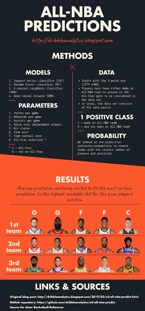
Summary
Below is an inforgraphic that presents a summary of the process and results.
Hi Tal, I'm very impressed with your work. Question: In 1999 the All Star Game was cancelled and first-time All-NBA team selects Alonzo Mourning, Allen Iverson, Jason Kidd, Chris Webber, Kevin Garnett, Antonio McDyess, and Kobe Bryant would have been left out of your model (if you are running a prediction for 1999 using previous years as a training set). Do you think this affects your model? How would you change it to account for the 3% that have never been all-star or all-nba selection before? Particularly important because the guys listed above are not only Hall Of Famers, they are some of the best to play the game – feels wrong to leave em out of the algorithm.
EDIT: Just Iverson and MCDyess would be left out because others had been All-Stars in the past
Thanks for checking it out.
I don't think missing out on the 1999 All-Star game affects the model a lot. Like you mentioned, it's only about 3% of the data. Though it would be better to have that data, given that there are already about 1,000 data points, I'm not sure if 25 more would make a drastic difference. The fact that Iverson and McDyess were left out wouldn't matter much on the stats side. The models don't know player names, reputation, etc. – they just know stats.
Thanks!